Video Introduction to ROI Analyses

About forty years ago certain persons went up to Laputa, either upon business or diversion, and upon their return began to dislike the management of everything below, and fell into schemes of putting all arts, sciences, languages, and mechanics upon a new foot. To this end they procured a royal patent for erecting an Academy of Projectors in Lagado. Every room hath in it one or more projectors. The first man I saw had been eight years extracting sunbeams out of cucumbers.

--Swift: Gulliver's Travels, Part III, chs. 4-5


I'm updating my videos on fMRI basics, starting with ROI analysis. This is low-hanging fruit, yes, but delicious fruit, fruit packed with nutrients and sugars and vitamins and knowledge, fruit that will cure the scurvy of ignorance and halt the spreading gangrene of frustration.

In these videos you will observe a greater emphasis on illustration and analogy, two of the most effective ways to have concepts like ROI analysis take root inside your mind; to make them have a real, visceral presence when you think about them, and not to exist merely as words that happened to impinge on your retina. These videos take longer to make, but are all the more rewarding. And if they help you to think differently than you did before, if they help you, even without my knowing it, to see the world as I understand it, then I will have taken a significant step toward fulfilling my purpose here on this earth.

Getting Started with E-Prime, Chapter 1: Objects

When I first opened up E-Prime, the experiment builder, I was struck by how colorful it was: the thumbnails of flags, hourglasses, computer screens; the blocks of code in shades of blues, greens, and grays; and, especially charming, the outline of a little purple man running, a cute way to represent the "run" button - yet to develop associations of errors, troubleshooting, and failure. Always watching, always waiting, perpetually frozen in running profile, was the little purple man, future inhabitant of future nightmares.

All of these colors led me to believe that E-Prime was a friendly software package for the non-programmer, and that it would definitely not lead to feelings of worthlessness, frustration, and eating an entire Sara Lee cake. However, I was proved wrong when I had to make an experiment more complicated than displaying the words "Hello," "Goodbye," and possibly loading a video file of a dog burping. (This can be found with your E-Prime installation under My Experiments/DogBurp_Demo.es2.) Which is how I came upon the E-Prime documentation.

The documentation for E-Prime is big. I recommend printing it, stapling it together with an industrial-sized Kirkland stapler from Costco, and feeling its heft. Or, if you prefer not to print it, open it up in a word processor and see how the scrollbar shrinks to the size of a tic-tac. In both cases the feeling is the same: This thing is Big. Huge. Biggest thing ever.

And then there are the words - the words! Words like object, procedure, list; context, attribute, trial; dimension, property, sphincter, photosynthesis. For someone with no coding background, this is a strange argot - words familiar in everyday life, but hopelessly confusing when trying to build an experiment. No wonder so many graduate students lose faith, drop out of school, and, instead of pursuing the invigorating career of a researcher spending the majority of his life in front of a computer, they wind up in some dull, unexciting job, such as professional gambler or hitman.

I don't want you to suffer the same fate. This is the start of my own documentation for E-Prime: An alternative to the Youtube videos posted by PST, the company that spawned E-Prime, and its bastard, slack-titted gorgon half-sister, E-Basic. I find those videos well-meaning and sometimes informative, but incomplete. After all, they were made by the programmers of E-Prime - they didn't have to slave away at it, suffer for it, like you and I did! This is my perspective from the other side; recognizing the typical pitfalls awaiting a new programmer and how to avoid them, along with how to make E-Prime submit to your will. The solutions are not always elegant; the coding will infuriate; but, if you watch the videos, you just might get the answers you need. No school this afterlunch, but education certain, with Andy as teacher.

Bayesian Inference Web App That Explains (Nearly) Everything

For those still struggling to understand the concepts of Bayesian inference - in other words, all of you - there is a web app developed by Rasmus Baath which allows one to see the process unfolding in real time. Similar to an independent-samples t-test, we are trying to estimate a parameter of the mean difference between the populations that the samples were drawn from; however, the Bayesian approach offers much richer information about a distribution of parameter values, and, more importantly, which ones are more credible than others, given the data that has been collected.

The web app is simple to use: You input data values for your two groups, specify the number of samples and burn-in samples (although the defaults for this are fine), and then hit the Start button. The MCMC chain begins sampling the posterior distribution, which builds up a distribution of credible parameter values, and 95% of the distribution containing the parameter values with the most credibility is labeled as the highest density interval, or HDI. This same procedure is applied to all of the other parameters informed by the data, including normality, effect size, and individual group means and standard deviations, which provides a much richer set of information than null hypothesis significance testing (NHST).

Because of this I plan to start incorporating more Bayesian statistics into my posts, and also because I believe it will overtake, replace, and destroy NHST as the dominant statistical method in the next ten years, burning its crops, sowing salt in its fields, looting its stores, stampeding its women, and ravishing its cattle. All of this, coming from someone slated to teach the traditional NHST approach next semester; which, understandably, has me conflicted. On the one hand, I feel pressured to do to whatever is most popular at the moment; but on the other, I am an opportunistic coward.

In any case, Bayesian inference is becoming a more tractable technique, thanks to programs that interface with the statistics package R, such such JAGS. Using this to estimate parameters for region of interest data, I think, will be a good first step for introducing Bayesian methods to neuroimagers.

DTI Analysis: Soup to Nuts Playlist

Instead of going through each DTI analysis step individually, I've collated everything into a Youtube playlist down below. Just remember that we are using data from the FSL practical course here, and also remember that suing somebody for giving out bad advice, although it is admittedly an easy way to become fantastically wealthy, won't necessarily make you happier.

In any case, just to briefly go over the rest of the steps: After correcting for magnetic field distortions and eddy currents, tensors are fitted using the dtifit command (or simply going through the FDT menu in the FSL interface). Once this has been done for each subject, a series of TBSS tools are used, each one prefixed by "tbss"; for example, tbss_1_preproc, tbss_2_reg, and so on. (You can find all of these in the $FSLDIR/bin directory, and if you have a good handle on Unix programming, you can inspect the code yourself.) After you have run all of those for your dataset, you set up the appropriate experimental design and contrasts, and use the randomise tool to perform statistics in your tractography mask.

Keep in mind that this is just beginner's material; and that if you were to compare your DTI competence to dating, if would be like you were still in that awkward teenager phase, unable to talk to anybody or make eye contact.

However, much of this material has already been covered in other blogs and online resources, provided by several other highly talented scientists and researchers, and - as much as I constantly fantasize about establishing a monopoly over neuroimaging information - there is no practical way to destroy them all.

Therefore, instead of posting redundant information, I highly recommend checking out an ongoing step-by-step series on TORTOISE by Peter Molfese, which you can compare to your results with FSL, and another blog dedicated to diffusion imaging, diffusion-imaging.com. The latter site covers virtually every piece of diffusion imaging software and pipeline out there, and is a good place to start.

Independent Components Analysis, Part II: Using FSL Example Data

For our next step, we will be working with FSL example data - somewhat artificial data, true, and much better quality than anything you can ever expect from the likes of your data, which will only lead to toil, sweat, and the garret. Sufficient unto the day is the frustration thereof.

However, it is a necessary step to see what ICA analysis ought to look like, as well as learning how to examine and identify components related to tasks and networks that you are interested in. Also - and possibly more important - you will learn to recognize sources of noise, such as components related to head motion and physiological artifacts.

First, go to the link http://fsl.fmrib.ox.ac.uk/fslcourse/ and scroll to the bottom for instructions on how to download the datasets. You can use either wget or curl. For this demonstration, we will be using datasets 2 and 6:

curl -# -O -C - http://fsl.fmrib.ox.ac.uk/fslcourse/fsl_course_data2.tar.gz

curl -# -O -C - http://fsl.fmrib.ox.ac.uk/fslcourse/fsl_course_data6.tar.gz

Once you have downloaded them, unzip them using gunzip, and then "tar -xf" on the resulting tar files. This will create a folder called fsl_course_data, which you should rename so that they do not conflict with each other. Within fsl_course_data2, navigate to the /melodic/av directory, where you will find a small functional dataset that was acquired while the participant was exposed to auditory stimuli and visual stimuli - which sounds much more scientific than saying, "The participant saw stuff and heard stuff."

Open up the MELODIC gui either through the FSL gui, or through typing Melodic_gui from the command line. Most of the preprocessing steps can be kept as is. However, keep the following points in mind:

1. Double-check the TR. FSL will fill it in automatically from the header of the NIFTI file, but it isn't always reliable.

2. Spatial smoothing isn't required in ICA, but a small amount can help produce better-looking and more identifiable component maps. Somewhere on the order of the size of a voxel or two will usually suffice.

3. By default, MELODIC automatically estimates the number of components for you. However, if you have severe delusions and believe that you know how many components should be generated, you can turn off the "Automatic dimensionality estimation" option in the Stats tab, and enter the number of components you want.

4. The Threshold IC maps option is not the same thing as a p-value correction threshold. I'm not entirely clear on how it relates to the mixture modeling carried out by ICA, but my sense from reading the documentation and papers using ICA is that a higher threshold only keeps those voxels that have a higher probability of belonging to the true signal distribution, instead of the background noise distribution, and it comes down to a balance between false positives and false negatives. I don't have any clear guidelines about what threshold to use, but I've seen cutoffs used within the 0.8-0.9 range in papers.

5. I don't consider myself a snob, but I was using the bathroom at a friend's house recently, and I realized how uncomfortable that cheap, non-quilted toilet paper can be. It's like performing intimate hygiene with roofing materials.

6. Once you have your components, you can load them into FSLview and scroll through them with the "Volumes" button in the lower left corner. You can also load the Atlases from the Tools menu and double-click on it to get a semi-transparent highlight of where different cortical regions are. This can be useful when trying to determine whether certain components fall within network areas that you would expect them to.

More details in the videos below, separately for the visual-auditory and resting-state datasets.

Regional Homogeneity Analysis with 3dReHo, Part 1: Introduction

Learning a new method, such as regional homogeneity analysis, can be quite difficult, and one often asks whether there is an easier, quicker method to become enlightened. Unfortunately, such learning can only be accomplished through large, dense books. Specifically, you should go to the library, check out the largest, heaviest book on regional homogeneity analysis you can find, and then go to the lab of someone smarter than you and threaten to smash their computer with the book unless they do the analysis for you.

If for some reason that isn't an option, the next best way is to read how others have implemented the same analysis; such as me, for example. Just because I haven't published anything on this method, and just because I am learning it for the first time, doesn't mean you should go do something rash, such as try to figure it out on your own. Rather, come along as we attempt to unravel the intriguing mystery of regional homogeneity analysis, and hide from irate postdocs whose computers we have destroyed. In addition to the thrills and danger of finding things out, if you follow all of the steps outlined in this multi-part series, I promise that you will be the first one to learn this technique from a blog. And surely, that must count for something.

With regional homogeneity analysis (or ReHo), researchers ask similar questions as with functional connectivity analysis; however, in the case of ReHo, we correlate the timecourse in one voxel with its immediate neighbors, or with a range of neighbors within a specified radius, instead of using a single voxel or seed region and testing for correlations with every other voxel in the brain, as in standard functional connectivity analysis.

As an analogy, think of ReHo as searching for similarities in the timecourse of the day's temperature between different counties across a country. One area's temperature timecourse will be highly correlated with neighboring counties's temperatures, and the similarity will tend to decrease the further away you go from the county you started in. Functional connectivity analysis, on the other hand, looks at any other county that shows a similar temperature timecourse to the county you are currently in.

Similarly, when ReHo is applied to functional data, we look for differences in local connectivity; that is, whether there are differences in connectivity within small areas or cortical regions. For example, when comparing patient groups to control groups, there may be significantly less or significantly more functional connectivity in anterior and posterior cingulate areas, possibly pointing towards some deficiency or overexcitation of communication within those areas. (Note that any differences found in any brain area with the patient group implies that there is obviously something "wrong" with that particular area compared to the control group, and that the opposite can never be true. While I stand behind this arbitrary judgment one hundred percent, I would also appreciate it if you never quoted me on this.)

As with the preprocessing step of smoothing, ReHo is applied to all voxels simultaneously, and that the corresponding correlation statistic in each voxel quantifies how much it correlates with its neighboring voxels. This correlation statistic is called Kendall's W, and ranges between 0 (no correlation at all between the specified voxel and its neighbors) and 1 (perfect correlation with all neighbors). Once these maps are generated, they can then be normalized and entered into t-tests, producing similar maps that we used with our functional connectivity analysis.

Now that we have covered this technique in outline, in our next post we will move on to the second, more difficult part: Kidnapping a senior research assistant and forcing him to do the analysis for us.

No, wait! What I meant was, we will review some papers that have used ReHo, and attempt to apply the same steps to our own analysis. If you have already downloaded and processed the KKI data that we used for our previous tutorial on functional connectivity, we will be applying a slightly different variation to create our ReHo analysis stream - one which will, I hope, not include federal crimes or destroying property.

Resting-State Functional Connectivity Analysis, Part II: Setting Up Your Analysis

Once you have downloaded the KKI dataset discussed in the last resting-state post, you have most of what you need, sacrificial undergraduate RA notwithstanding. Also, as I mentioned, we will be using AFNI for this, specifically AFNI's uber_subject.py script which includes an option for preprocessing and analyzing resting-state data.

First, type uber_subject.py from your terminal to open up the GUI (rhymes with "whey"), and select the resting-state option from the preprocessing selections. This will automatically fill in a series of preprocessing steps which our AFNI overlords, in their wisdom, have decided is best for resting-state analyses. Of course, you can change this, but that would be an unbelievably stupid decision, on par with doing something like asking out your girlfriend's sister.

Notice that with resting-state experiments, we avoid several of the annoying, persnickety details endemic to typical FMRI experiments, such as having to actually design an experiment. You simply place the subject inside the scanner, set the scanner to 350 degrees, and leave it for ten minutes. When you come back, you will have a slightly charred piece of carbon that used to be a human being. After framing someone else, such as your FMRI technician, you should then realize that you are simply not cut out for actually carrying out a resting-state scan, and download someone else's data instead from the Internet like I recommended in the first place.

Notice that much of the preprocessing and setting up the design matrix is the similar to usual FMRI analyses. However, there is an important difference in the design matrix setup, because you do not have any tasks or events to model. Instead, the only things you need to model are potential sources of noise, which may include heart rate or respiration data, if you have it, and always motion data, since this can be an insidious confound in any FMRI analysis, but particularly for resting-state analyses.

The upshot of all this is that, whereas in a traditional FMRI analysis AFNI saves the beta estimates and contrasts to a statistics dataset and everything else that wasn't modeled into an error or residual dataset (usually labelled "errts+orig"), in resting-state analyses we are interested in everything that wasn't explicitly modeled - in other words, we will want to focus on what gets output to the errts+orig dataset, since that will contain the timecourses of voxel activity that we are interested in. You can then place ROIs or other seed regions within that dataset, and generate correlation maps from those seed regions.

In the next chapter of the series, we will look more closely at converting these correlation values into z-maps for comparison across groups, as well as where to find more undergraduate RAs if the ones who were working in your lab have already been burnt as offerings to the FMRI gods.

Creating Functional Connectivity Maps in AFNI (Second Step on the Road Towards Glory)

Having used 3dSynthesize to create a dataset with the effects of no interest, we are now ready to subtract those effects from the dataset that went into 3dDeconvolve; for you players using the AFNI_data6 tutorial data, this is the all_runs.FT+orig dataset. We can use 3dcalc for this operation:

3dcalc -a all_runs.FT+orig -b effectsNoInterest+orig -expr 'a-b' -prefix cleanData+orig

This will create a time series with all the drift correction and motion parameter schmutz subtracted out and cast into the pit. What is left over will be signal untainted by motion or drift effects, which we can then use to generate a seed time series.

Before that, however, there is the additional step of warping our data to a template space (such as MNI or Talairach). Assuming you have already warped your anatomical dataset to a template space either manually or using @auto_tlrc, and assuming that there is already good alignment between your anatomical and functional data, you can use the command adwarp:

adwarp -apar anat_final.FT+tlrc -dpar cleanData+orig -dxyz 3 -prefix EPI_subj_01

(Note: There are better ways to do warping, such as the warping option built into align_epi_anat.py (which calls upon @auto_tlrc), but for pedagogical purposes we will stick with adwarp.)

Once this is done, all we need to do is select a seed region for our functional connectivity analysis. This could be a single voxel, a region of interest that averages over an entire area of voxels, or a region selected based on a contrast or an anatomical landmark; it depends on your research question, or whether you want to mess around and do some exploratory analyses. For now, we will use a single voxel using XYZ coordinates centered on the left motor cortex (note that, in this coordinate system, left is positive and posterior is positive):

3dmaskdump -noijk -dbox 20 19 53 EPI_subj_01+tlrc > ideal_ts.1D

Because 3dmaskdump outputs a single row, we will need to transpose this into a column:

1dtranspose ideal_ts.1D LeftMotorIdeal.1D

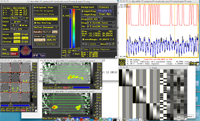
After you have output your ideal timeseries, open up the AFNI viewer and make sure that what was output matches up with the actual timeseries. In this example, set EPI_subj_01+tlrc as an underlay and right click in the slices viewer to jump to XYZ coordinates of 20, 19, 53; open up the timeseries graph as well, and scroll to the first time point. Does the value there match up with the first entry of your ideal time file? If not, you may have mis-specified the voxel you wanted, or you are using a different XYZ grid than is displayed in the upper left corner of the AFNI viewer. If you run into this situation, consult your local AFNI guru; if you don't have one of those, well...

In any case, we now have all the ingredients for the functional connectivity analysis, and we're ready to pull the trigger. Assemble your materials using 3dfim+ (which, as far as I can understand, stands for "functional intensity map," or something like that):

3dfim+ -polort 3 -input EPI_subj_01+tlrc -ideal_file LeftMotorIdeal.1D -out Correlation -bucket Corr_subj01

You will now have a dataset, Corr_subj_01+tlrc, which is a functional connectivity map between your seed region and the rest of the brain. Note that the threshold slider will now be in R values, instead of beta coefficients or t-statistics; therefore, make sure the order of magnitude button (next to the '**' below the slider) is 0, to restrict the range between +1 and -1.

The last step is to convert these correlation values into z-scores, to reduce skewness and make the distribution more normal. This is done through Fisher's R-to-Z transformation, given by the formula z =  (1/2) * ln((1+r)/(1-r)). Using 3dcalc, we can apply this transformation:

3dcalc -a Corr_subj01+tlrc -expr 'log((1+a)/(1-a))/2' -prefix Corr_subj01_Z+tlrc

Those Z-maps can then be entered into a second-level design just like any other, using 3dttest+ or some other variation.

Sanity check: When viewing the correlation maps, jump to your seed region and observe the r-value. It should be 1, which makes sense given that this was the region we were correlating with every other part of the brain, and correlating it with itself should be perfect.

Like me.

AFNI Start to Finish Playlist

Although the title may sound a little risqué, what it actually refers to is a compilation of tutorials - twenty-one in all - that cover the analysis of a single subject from data import to viewing the results and making publication-quality pictures. I closely follow a script already up on the AFNI website written by Rick Reynolds, and I've included links to the relevant step of the script. The idea here was to actually show what each step looks like, and to provide some additional commentary. Half of the commentary is wrong, though; the only problem is, I'm not sure which half.

A link to the script can be found here; a link to the tutorials can be found here. Particularly important is understanding the design matrix, and gaining an intuition for how it is applied at each voxel; I will be going into more detail about that in the future.

AFNI Command: 3dUnifize

Are you disgusted with the way your T1-weighted images look? Trying to reduce the intensity imbalance in your anatomical? When your friends tell you that your structural looks "fine", do you find yourself not really believing them? If so, then 3dUnifize can help. Simply supply a prefix for the output dataset and the name of your anatomical image, and thirty seconds later you have a relatively balanced T1 image.

To be honest, probably very few, if any, people will use this program. However, it does draw attention to the ability to look up and check on intensity values of your images, as this can be a useful diagnostic tool in some cases. Once you've loaded up the AFNI GUI click on the Overlay tab and look at the values to the right of the ULay (Underlay) and OLay (Overlay) labels. These will provide the intensity of the image, whether in arbitrary units - for example, if you had a raw T1- or T2-weighted image loaded - or statistical values, such as when you overlay a t-map.

Also, due to a recent purge in the lab, I am now officially moved in to a new office. More exciting details about my life, plus an obnoxiously loud computer fan, can be found in the following video.