|
| Different sized smoothing kernels applied to a functional dataset. Note that larger smoothing kernels cause a loss of spatial resolution by turning the relatively high resolution, jagged-edged dataset in the upper left, into the soft, puffy, amorphous cotton ball in the lower right. |
Smoothing is one of the most straightforward processing steps, simply involving the application of spatial filtering to your data. Signal is averaged over a range of nearby voxels in order to produce a new estimate of the signal at each voxel, and the range can be narrowed or extended to whatever range suits the researcher's delectation. It is rare for this step to fail, as it is not contingent on overlapping modalities; nor is it susceptible to typical neuroimaging landmines such as entrapment in local minima. Furthermore, the benefits are several: True signal tends to be amplified while noise is canceled out, and power is therefore increased. As a result, often this step is thrown in almost as an afterthought, the defaults left flicked into the "On" position, and quickly forgotten about, as the researcher scampers out of the lab and into his Prius for a quick connection before dinner.
However, smoothing can also be deceptively treacherous. For those researchers intending to tease apart discrete cortical or subcortical regions - for example, the amygdala, if you're into that kind of thing - will find that smoothing tends to smear signal across a wide area, leading to a reduction in spatial specificity. Furthermore, ridiculously large smoothing kernels can actually lead to lower t-values in peak voxels. This may appear to be counterintuitive at first; however, note that increasing the range of voxels can begin to recruit voxels which have nothing to do with the signal you are looking at, and can even begin to average signal from voxels which have an opposite deflection to the signal you are interested in.
 |
| Effect
of smoothing kernels on statistical results. Here, a contrast of
left-right was performed on datasets smoothed with a 4mm kernel. Note
that as the smoothing kernel increases, the peak t-value decreases, as depicted by the thermometer bar. |
 |
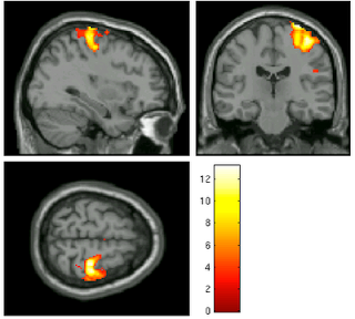
| 8mm kernel |
 |
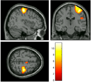
| 15mm kernel |
For example, let's say we are interested in the contrast of left button presses minus right button presses, as pictured above; as we increased the smoothing kernel, more and more voxels become part of the big blog - I mean, blob! - and it appears that our power increases as well. However, as we extend our averaging over a wider expanse over the fields and prairies of voxels, we risk beginning to smooth in signal from white matter and increasingly unrelated areas. At the most extreme, one can imagine smoothing in signal from the opposite motor cortex, which, for this contrast, will have strongly negative beta estimates.
Your sensitive FMRI antennae should also be attuned to the fact that smoothing can be applied at different magnitudes in the x-, y-, and z-directions. For example, if you are particularly twisted, you could smooth eight millimeters in the y- and z-directions, but only six millimeters in the x-direction. This also comes into play when estimating the smoothness of a first- or second-level analysis, as the smoothing extent may differ along all three coordinates.
For more details, along with a sample of my writing style as a younger man, see the following posts:
Group Level Smoothness Estimation in SPM
Smoothing in AFNI