Video Introduction to ROI Analyses


About forty years ago certain persons went up to Laputa, either upon business or diversion, and upon their return began to dislike the management of everything below, and fell into schemes of putting all arts, sciences, languages, and mechanics upon a new foot. To this end they procured a royal patent for erecting an Academy of Projectors in Lagado. Every room hath in it one or more projectors. The first man I saw had been eight years extracting sunbeams out of cucumbers.

--Swift: Gulliver's Travels, Part III, chs. 4-5


I'm updating my videos on fMRI basics, starting with ROI analysis. This is low-hanging fruit, yes, but delicious fruit, fruit packed with nutrients and sugars and vitamins and knowledge, fruit that will cure the scurvy of ignorance and halt the spreading gangrene of frustration.

In these videos you will observe a greater emphasis on illustration and analogy, two of the most effective ways to have concepts like ROI analysis take root inside your mind; to make them have a real, visceral presence when you think about them, and not to exist merely as words that happened to impinge on your retina. These videos take longer to make, but are all the more rewarding. And if they help you to think differently than you did before, if they help you, even without my knowing it, to see the world as I understand it, then I will have taken a significant step toward fulfilling my purpose here on this earth.

SPM Smoothing: A Reader Writes

The angry red pustule of the Gaussian normal distribution
I love questions, because questions get answers. One question you may be asking is, "Why are my smoothness estimates in SPM so whack?" To which the obvious response is, "How much whack are we talking about here? Whiggidy-whack, or just the regular kind?" Details matter.

If the former, then the following code snippet may help. In the absence of a gold standard for calculating smoothness estimates, often we have to resort to our own ingenuity and cunning, by which I mean: Copy what other people are doing. One alert reader, Tamara, noticed that the standard SPM function for estimating smoothness, spm_est_smoothness, is so whack that all the other SPM functions want nothing to do with it. Which is kind of the goal of life, when you think about it - to not be that guy everyone else wants to avoid.

In any case, if you are having issues with it, the following code may help. I've also included the rest of the email, just to make you aware that I can and will publish your correspondence without your consent.


Hi Andy, I never figured out why spm_est_smoothness is not working, although other people have had the same issue with getting estimates in the thousands.  Ultimately, I ended up using this simple code to estimate each individual's smoothness, and then averaged across subjects.  Jim Lee posted this on the SPM listserv along with this note:  
The smoothness estimates in SPM.xVol.FWHM are in units of VOXELS, so you need to multiply by the voxel dimensions to get them in mm. Something like this:
load SPM.mat; M = SPM.xVol.M; VOX = sqrt(diag(M(1:3,1:3)'*M(1:3,1:3)))'; FWHM = SPM.xVol.FWHM; FWHMmm= FWHM.*VOX; disp(FWHMmm);

Thanks again for your help!!

Converting T-Maps to Z-Maps

Mankind craves unity - the peace that comes with knowing that everyone thinks and feels the same. Religious, political, social endeavors have all been directed toward this same end; that all men have the same worldview, the same Weltanschauung. Petty squabbles about things such as guns and abortion matter little when compared to the aim of these architects. See, for example, the deep penetration into our bloodstream by words such as equality, lifestyle, value - words of tremendous import, triggering automatic and powerful reactions without our quite knowing why, and with only a dim awareness of where these words came from. That we use and respond to them constantly is one of the most astounding triumphs of modern times; that we could even judge whether this is a good or bad thing has already been rendered moot. Best not to try.

It is only fitting, therefore, that we as neuroimagers all "get on the same page" and learn "the right way to do things," and, when possible, make "air quotes." This is another way of saying that this blog is an undisguised attempt to dominate the thoughts and soul of every neuroimager - in short, to ensure unity. And I can think of no greater emblem of unity than the normal distribution, also known as the Z-distribution - the end, the omega, the seal of all distributions. The most vicious of arguments, the most controversial of ideas are quickly resolved by appeal to this monolith; it towers over all research questions like a baleful phallus.

There will be no end to bantering about whether to abolish the arbitrary nature of p less than 0.05, but the bantering will be just that. The standard exists for a reason - it is clear, simple, understood by nearly everyone involved, and is as good a standard as any. A multitude of standards, a deviation from what has become so steeped in tradition, would be chaos, mayhem, a catastrophe. Again, best not to try.

I wish to clear away your childish notions that the Z-distribution is unfair or silly. On the contrary, it will dominate your research life until the day you die. Best to get along with it. The following SPM code will allow you to do just that - convert any output to the normal distribution, so that your results can be understood by anyone. Even by those who disagree, or wish to disagree, with the nature of this thing, will be forced to accept it. A shared Weltanschauung is a powerful thing. The most powerful.


=============

The following Matlab snippet was created by my adviser, Josh Brown. I take no credit for it, but I use it frequently, and believe others will get some use out of it. The calculators in each of the major statistical packages - SPM, AFNI, FSL - all do the same thing, and this is merely one application of it. The more one gets used to applying these transformations to achieve a desired result, the more intuitive it becomes to work with the data at any stage - registration, normalization, statistics, all.


%
% Usage:  convert_spm_stat(conversion, infile, outfile, dof)
%
% This script uses a template .mat batch script object to
% convert an SPM (e.g. SPMT_0001.hdr,img) to a different statistical rep.
% (Requires matlab stats toolbox)
%
%  Args:
%  conversion -- one of 'TtoZ', 'ZtoT', '-log10PtoZ', 'Zto-log10P',
%               'PtoZ', 'ZtoP'
%  infile -- input file stem (may include full path)
%  outfile -- output file stem (may include full pasth)
%  dof -- degrees of freedom
%
% Created by:           Josh Brown 
% Modification date:    Aug. 3, 2007
% Modified: 8/21/2009 Adam Krawitz - Added '-log10PtoZ' and 'Zto-log10P'
% Modified: 2/10/2010 Adam Krawitz - Added 'PtoZ' and 'ZtoP'

function completed=convert_spm_stat(conversion, infile, outfile, dof)

old_dir = cd();

if strcmp(conversion,'TtoZ')
    expval = ['norminv(tcdf(i1,' num2str(dof) '),0,1)'];
elseif strcmp(conversion,'ZtoT')
    expval = ['tinv(normcdf(i1,0,1),' num2str(dof) ')'];
elseif strcmp(conversion,'-log10PtoZ')
    expval = 'norminv(1-10.^(-i1),0,1)';
elseif strcmp(conversion,'Zto-log10P')
    expval = '-log10(1-normcdf(i1,0,1))';
elseif strcmp(conversion,'PtoZ')
    expval = 'norminv(1-i1,0,1)';
elseif strcmp(conversion,'ZtoP')
    expval = '1-normcdf(i1,0,1)';
else
    disp(['Conversion "' conversion '" unrecognized']);
    return;
end
    
if isempty(outfile)
    outfile = [infile '_' conversion];
end

if strcmp(conversion,'ZtoT')
    expval = ['tinv(normcdf(i1,0,1),' num2str(dof) ')'];
elseif strcmp(conversion,'-log10PtoZ')
    expval = 'norminv(1-10.^(-i1),0,1)';
end

%%% Now load into template and run
jobs{1}.util{1}.imcalc.input{1}=[infile '.img,1'];
jobs{1}.util{1}.imcalc.output=[outfile '.img'];
jobs{1}.util{1}.imcalc.expression=expval;

% run it:
spm_jobman('run', jobs);

cd(old_dir)
disp(['Conversion ' conversion ' complete.']);
completed = 1;


Assuming you have a T-map generated by SPM, and 25 subjects that went into the analysis, a sample command might be:

convert_spm_stat('TtoZ', 'spmT_0001', 'spmZ_0001', '24')

Note that the last argument is degrees of freedom, or N-1.


Slice Analysis of FMRI Data with SPM


Slice analysis is a simple procedure - first you take a jar of peanut butter and a jar of Nutella, and then use a spoon to take some Nutella and then use the same spoon to mix it with the peanut butter. Eat and repeat until you go into insulin shock, and then...

No, wait! I was describing my midnight snack. The actual slice analysis method, although less delicious, is infinitely more helpful in determining regional dissociations of activity, as well as avoiding diabetes. (Although who says they can't both be done at the same time?)

The first step is to extract contrast estimates for each slice from a region of interest (ROI, also pronounced "ROY") and then average across all the voxels in that slice for the subject. Of course, there is no way you would be able to do this step on your own, so we need to copy someone else's code from the Internet and adapt it to our needs; one of John Ashburner's code snippets (#23, found here) is a good template to start with. Here is my adaptation:


rootdir = '/data/drill/space10/PainStudy/fmri/'; %Change these to reflect your directory structure
glmdir = '/RESULTS/model_RTreg/'; %Path to SPM.mat and mask files

subjects = [202:209 211:215 217 219 220:222 224:227 229 230 232 233];
%subjects = 202:203;

Conditions.names = {'stroopSurpriseConStats', 'painSurpriseConStats'}; %Replace with your own conditions
Masks = {'stroopSurpriseMask.img', 'painSurpriseMask.img'}; %Replace with your own masks; should be the product of a binary ROI multiplied by your contrast of interest
Conditions.Contrasts = {'', ''};

ConStats = [];
Condition1 = [];
Condition2 = [];

for i=subjects
    
    cd([rootdir num2str(i) glmdir])
    outputPath = [rootdir num2str(i) glmdir]; %Should contain both SPM.mat file and mask files
    
    for maskIdx = 1:length(Masks)
      
    P = [outputPath Masks{(maskIdx)}];

    V=spm_vol(P);

    tmp2 = [];
    
     [x,y,z] = ndgrid(1:V.dim(1),1:V.dim(2),0);
     for i=1:V.dim(3),
       z   = z + 1;
       tmp = spm_sample_vol(V,x,y,z,0);
       msk = find(tmp~=0 & isfinite(tmp));
       if ~isempty(msk),
         tmp = tmp(msk);
         xyz1=[x(msk)'; y(msk)'; z(msk)'; ones(1,length(msk))];
         xyzt=V.mat(1:3,:)*xyz1;
         for j=1:length(tmp),
           tmp2 = [tmp2; xyzt(1,j), xyzt(2,j), xyzt(3,j), tmp(j)];
         end;
       end;
     end;

         xyzStats = sortrows(tmp2,2); %Sort relative to second column (Y column); 1 = X, 3 = Z
         minY = min(xyzStats(:,2));
         maxY = max(xyzStats(:,2));

         ConStats = [];

     for idx = minY:2:maxY
         x = find(xyzStats(:,2)==idx); %Go in increments of 2, since most images are warped to this dimension; however, change if resolution is different
         ConStats = [ConStats; mean(xyzStats(min(x):max(x),4))];
     end

    if maskIdx == 1
        Condition1 = [ConStats Condition1];
    elseif maskIdx == 2
        Condition2 = [ConStats Condition2];
    end

    end
end

Conditions.Contrasts{1} = Condition1;
Conditions.Contrasts{2} = Condition2;


This script assumes that there are only two conditions; more can be added, but care should be taken to reflect this, especially with the if/else statement near the end of the script. I could refine it to work with any amount of conditions, but that would require effort and talent.

Once these contrasts are loaded into your structure, you can then put them in an Excel spreadsheet or any other program that will allow you to format and save the contrasts in a tab-delimited text format. The goal is to prepare them for analysis in R, where you can test for main effects and interactions across the ROI for your contrasts. In Excel, I like to format it in the following four-column format:


Subject Condition Position  Contrast
202 Stroop 0 -0.791985669
202 Stroop 2 -0.558366941
202 Stroop 4 -0.338829942
202 Pain 0 0.17158524
202 Pain 2 0.267789503
202 Pain 4 0.192473782
203 Stroop 0 0.596162455
203 Stroop 2 0.44917655
203 Stroop 4 0.410870348
203 Pain 0 0.722974284
203 Pain 2 0.871030304
203 Pain 4 1.045700207


And so on, depending on how many subjects, conditions, and slices you have. (Note here that I have position in millimeters from the origin in the y-direction; this will depend on your standardized space resolution, which in this case is 2mm per slice.)

Once you export that to a tab-delimited text file, you can then read it into R and analyze it with code like the following:

setwd("~/Desktop")
x = read.table("SliceAnalysis.txt", header=TRUE)
x$Subject <- as.factor="" font="" ubject="" x="">
aov.x = aov(Contrast~(Condition*Position)+Error(Subject/(Condition*Position)),x)
summary(aov.x)
interaction.plot(x$Position, x$Condition, x$Contrast)


This will output statistics for main effects and interactions, as well as plotting the contrasts against each other as a function of position.

That's it! Enjoy your slices, crack open some jars of sugary products, and have some wild times!


Automating SPM Contrasts

Manually typing in contrasts in SPM is a grueling process that can have a wide array of unpleasant side effects, including diplopia, lumbago, carpal tunnel syndrome, psychosis, violent auditory and visual hallucinations, hives, and dry mouth. These symptoms are only compounded by the number of regressors in your model, and the number of subjects in your study.

Fortunately, there is a simply way to automate all of this - provided that each subject has the same number of runs, and that the regressors in each run are structured the same way. If they are, though, the following approach will work.

First, open up SPM and click on the TASKS button in the upper right corner of the Graphics window. The button is marked "TASKS" in capital letters, because they really, really want you to use this thing, and mitigate all of the damage and harm in your life caused by doing things manually. You then select the Stats menu, then Contrast Manager. The options from there are straightforward, similar to what you would do when opening up the Results section from the GUI and typing in contrasts manually.

When specifying the contrast vector, take note of how many runs there are per subject. This is because we want to take the average parameter estimate for each regressor we are considering; one can imagine a scenario where one of the regressors occurs in every run, but the other regressor only happens in a subset of runs, and this more or less puts them on equal footing. In addition, comparing the average parameter or contrast estimate across subjects is easier to interpret.

Once you have the settings to your satisfaction, save it out as a .mat file - for example, 'RunContrasts.mat'. This can then be loaded from the command line:

load('RunContrasts')

Which will put a structure called "jobs" in your workspace, which contains all of the code needed to run a first-level contrast. The only part of it we need to change when looping over subjects is the spmmat field, which can be done with code like the following:

subjList=[207 208]; %And so on, including however many subjects you want

for subj=subjList

    jobs{1}.stats{1}.con.spmmat =     {['/data/hammer/space4/MultiOutcome2/fmri/' num2str(subj) '/RESULTS/model_multiSess/SPM.mat']} %This could be modified so that the path is a variable reflecting where you put your SPM.mat file
    spm_jobman('run', jobs)

end

This is demonstrated in the following pair of videos; the first, showing the general setup, and the second showing the execution from the command line.


Parametric Modulation with SPM: Why Order Matters

Those who are the youngest children in the family are keenly aware of the disadvantages of being last in the pecking order; the quality of toys, clothes, and nutrition is often best for the eldest children in the family, and gradually tapers off as you reach the last kids, who are usually left with what are called, in parent euphemisms, "hand-me-downs."

In reality, these are things that should have been discarded several years ago due to being broken, unsafe, containing asbestos, or clearly being overused, such as pairs of underwear that have several holes in them so large that you're unsure of where exactly your legs go.

In SPM land, a similar thing happens to parametric modulators, with later modulators getting the dregs of the variance not wanted by the first modulators. Think of variance as toys and cake, and parametric modulators as children; everybody wants the most variance, but only the first modulators get the lion's share of it; the last modulators get whatever wasn't given to the first modulators.

The reason this happens is because when GLMs are set up, SPM uses a command, spm_orth, to orthogonalize the modulators. The first modulator is essentially untouched, but all other modulators coming after it are orthogonalized with respect to the first; and this proceeds in a stepwise function, with the second modulator getting whatever was unassigned to the first, the third getting whatever was unassigned to the second, and so on.

(You can see this for yourself by doing a couple of quick simulations in Matlab. Type x1=rand(10,1), and x2=rand(10,1), and then combine the two into a matrix with xMat = [x1 x2]. Type spm_orth(xMat), and notice that the first column is unchanged, while the second is greatly altered. You can then flip it around by creating another matrix, xMatRev = [x2 x1], and using spm_orth again to see what effect this change has.)

Be aware of this, as this can dramatically alter your results depending on how your modulators were ordered. (If they were completely orthogonal by design, then the spm_orth command should have virtually no impact; but this scenario is rare.) This came to my attention when looking at a contrast of a parametric modulator, which was one of three assigned to a main regressor. In one GLM, the modulator was last, and correspondingly explained almost no variance in the data; while in another GLM, the modulator was first, and loaded on much more of the brain. The following two figures show the difference, using exactly the same contrast and correction threshold, but simply reversing the order of the modulators:


Results window when parametric modulator was the last one in order.


Results window when parametric modulator was the first one in order.

This can be dealt with in a couple of ways:
  1. Comment out the spm_orth call in two scripts used in setting up the GLM: line 229 in spm_get_ons.m, and lines 285-287 in spm_fMRI_design.m. However, this might affect people who actually do want the orthogonalization on, and also this increases the probability that you will screw something up. Also note that doing this means that the modulators will not get de-meaned when entered into the GLM.
  2. Create your own modulators by de-meaning the regressor, inserting your value at the TR where the modulator occurred, then convolving this with an HRF (usually the one in SPM.xBF.bf). If needed, downsample the output to match the original TR.

It is well to be aware of all this, not only for your own contrasts, but to see how this is done in other papers. I recall reading one a long time ago - I can't remember the name - where several different models were used, in particular different models where the modulators were entered in different orders. Not surprisingly, the results were vastly different, although why this was the case wasn't clearly explained. Just something to keep in mind, as both a reader and a reviewer.

I should also point out that this orthogonalization does not occur in AFNI; the order of modulators has no influence on how they are estimated. A couple of simulations should help illustrate this:

Design matrices from AFNI with simulated data (one regressor, two parametric modulators.) Left: PM1 entered first, PM2 second. Right: Order reversed. The values are the same in both windows, just transposed to illustrate which one was first in the model.

More information on the topic can be found here, and detailed instructions on how to construct your own modulators can be found on Tor Wager's lab website.

Quick and Efficient ROI Analysis Using spm_get_data

For any young cognitive neuroscientist out for the main chance, ROI analyses are an indispensable part of the trade, along with having a cool, marketable name, such as Moon Unit or Dweezil Zappa. Therefore, you will find yourself doing a lot of such ROI analyses; and the quicker and more efficient you can do them, with a minimum of error, will allow you to succeed wildly and be able to embark upon an incredible, interesting career for the next four or five decades of your life before you die.

Most ROI analyses in SPM are carried out through the Marsbar toolbox, and for most researchers, that is all they will ever need. However, for those who feel more comfortable with the command line, there is a simple command within the SPM library - spm_get_data - that will make all of your ROI fantasies come true. All the command needs is an array of paths leading to the images you wish to extract data from, along with a matrix of coordinates representing the ROI.

First, the ROI coordinates can be gathered by loading up an arbitrary contrast and selecting an ROI created through, say, Marsbar or wfu_pickatlas. Next, set your corrected p-value threshold to 1; this will guarantee that every voxel in that ROI is "active," which will be recorded by a structure automatically generated each time the Results GUI is opened, a structure called xSPM. One of the fields, xSPM.XYZ, contains the coordinates for each voxel within that ROI. This can then be assigned to a variable, and the same procedure done for however many ROIs you have. The best part, however, is that you only need to do this once for each ROI; once you have assigned it to a variable, you can simply store it in a new .mat file with the "save" command (e.g., save('myROIs.mat', 'M1', 'ACC', 'V1')). These can then be restored to the Matlab workspace at any time by loading that .mat file.

Note: An alternative way to get these coordinates just from the command line would be the following:

Y = spm_read_vols(spm_vol(seedroi),1);
indx = find(Y>0);
[x,y,z] = ind2sub(size(Y),indx);

XYZ = [x y z]';

Where the variable "seedroi" can be looped over a cell containing the paths to each of your ROIs.


The next step is to create your array of images you wish to extract data from - which, conveniently, is stored within the SPM.mat file that is created any time you run a second-level analysis. For example, let's say that I carried out a couple of 2nd-level t-tests, one for left button presses, the other for right button presses. If I go into the folder for left button presses that has already estimated an run a second-level analysis, all of the contrast images that went into that analysis are now stored in SPM.xY.P, which is available in your workspace after simply navigating to the directory containing your SPM.mat file and typing "load SPM".

Lastly, spm_get_data is called to do the ROI analysis by extracting data from each voxel in the ROI for each subject for each contrast, and these are averaged across all of the voxels in that ROI using the "mean" function. Sticking with the current example, let's say have a left M1 region and a right M1 region, the coordinates of which have been extracted using the procedure detailed above, and which have been saved into variables called left_M1 and right_M1, respectively. I then navigate to the left button presses second-level directory, load SPM, and type the following command:

right_M1_leftButtonPress = mean(spm_get_data(SPM.xY.P, right_M1),2)

which returns an array of one value per subject for that contrast averaged across the ROI. You can then easily navigate to another second-level directory - say, right button presses - and, after loading the SPM.mat file, do the same thing:

right_M1_rightButtonPress = mean(spm_get_data(SPM.xY.P, right_M1),2)

T-tests can then be carried out between the sets of parameter or contrast estimates with the t_test function:

[h, p, ci, stats] = ttest(right_M1_leftButtonPress, right_M1_rightButtonPress)

which will return the p-value, confidence interval, and t-value that you would then report in your results.


Multiple Regression in SPM

A couple of videos have been posted about multiple regression in SPM, both at the first level and second level. Technically, almost all of the GLMs researchers usually set up use multiple linear regression, where a linear combination of weighted regressors is fit to the timecourse of each voxel. However, in SPM parlance, regressors are distinct from conditions: Conditions are typically convolved with some sort of basis function (usually a hemodynamic response function), whereas regressors are not convolved with anything. For example, someone may enter motion parameters as regressors, since they are not convolved with any hemodynamic shape, but still may account for some of the variance observed in the signal (and, we hope, the signal that is primarily due to motion). Another example would be entering in the timecourse extracted from an ROI to do a functional connectivity analysis, or inserting the interaction term from a PPI analysis as a regressor.

At the second level SPM also gives the option for doing multiple regression; but this is simply the entering of covariates which can be tested for correlations with the signal change in contrasts across subjects. In most cases, however, you can select any other design, and enter in covariates regardless of which design that you choose; which I believe to be the better option, since it is more flexible.

In any case, most of the rest of the details can be found in the following videos. Speak hands for me.


Updated SPM Command Line, Including Beta Series Option

I've updated the code of the previously discussed previous script in the previous post, previously, including the addition of more help text to explain certain options and termination of the script if the timing file is not found.

However, the biggest change is a block of code to convert the timings files so that each trial is now a regressor, before entering them into the GLM. With so many regressors, the GLM will look a little funky; possibly something like this:


Note that, since there are so many regressors and so many scans, not all of them are going to be labeled individually; but it should look as though there is only one estimation per column, or blip of white underneath each regressor. Also due to space constraints the parameter estimability may not be completely visible, but when each trial is being estimated individually, you should still get a beta for each trial. Check the output directory to make sure that you have the number of betas you think you should have: one for each trial, plus the amount of session constants (usually equal to the number of runs for the subject).

The updated script can be found here; as always, send me any comments if you encounter any serious issues or bugs. I recommend using it as a replacement for the previously discussed previous script, since it can either estimate each trial individually or average them together, depending on whether you set the DO_BETASERIES flag to 1 or 0.

All of this is explained clearly in the following video:


Running SPM First-Level Analyses from the Command Line

For most people, doing first-level analyses in SPM is tedious in the extreme; for other people, these analyses are manageable through command line scripting in Matlab. And there are still other people who don't even think about first-level analyses or SPM or Matlab or any of that. This last class of people are your college classmates who majored in something else, like economics, and are living significantly less stressful lives than you, making scads of money, and regularly eating out at restaurants where they serve shrimp the size of Mike Tyson's forearm.

Assuming that you belong to the first category, however, first-level analyses are invariably a crashing bore; and, worse, completely impractical for something like beta-series analysis, where a separate regressor is needed for individual events.

The following script will do all of that for you, although it makes many assumptions about your timing files and where everything is stored. First, your directory needs to be set up with a root directory containing all of the subjects, as well as a separate timing directory containing your onsets files; and second, that the timing files are written in a four-column format of runs, regressors, onsets (in seconds), and duration. Once you have all of that, though, all it takes is simply modifications of the script to run your analysis.

As always, let me know if this actually helps, or whether there are sections of code that can be cleaned up. I will be making a modification tomorrow allowing for beta series analysis by converting all of the timing events into individual regressors, which should help things out.

Link to script: http://mypage.iu.edu/~ajahn/docs/Run_SPM_FirstLevel.m

% INPUT:
%  rootDir        - Path to where subjects are located
%  subjects       - Vector containing list of subjects (can concatenate with brackets)
%  spmDir         - Path to folder where you want to move the multiple conditions .mat files and where to the output SPM file (directory is created if it doesn't
%  exist)
%  timingDir      - Path to timing directory, relative to rootDir
%  timingSuffix   - Suffix appended to timing files
%  matPrefix      - Will be prefixed to output .mat files.
%  dataDir        - Directory storing functional runs.
%
% OUTPUT:
%  One multiple condition .mat file per run. Also specifies the GLM and runs
%  beta estimation.
%       
%
%       Note that this script assumes that your timing files are organized
%       with columns in the following order: Run, ConditionName, Onset (in
%       seconds), Duration (in seconds)
%
%       Ideally, this timing file should be written out from your
%       presentation software, e.g., E-Prime
%
%       Also note how the directory tree is structured in the following example. You may have to
%       change this script to reflect your directory structure.
%       
%       Assume that:
%         rootdir = '/server/studyDirectory/'
%         spmDir = '/modelOutput/'
%         timingDir = '/timings/onsets/'
%         subjects = [101]
%         timingSuffix = '_timing.txt'
%       1) Sample path to SPM directory:
%       '/server/studyDirectory/101/modelOutput/'
%       2) Sample path to timing file in the timing directory:
%       '/server/studyDirectory/timings/onsets/101_timing.txt'
%
% Andrew Jahn, Indiana University, June 2014
% andysbrainblog.blogspot.com

clear all

%%%----Things you will want to change for your study----%%%

rootDir = '/data/hammer/space5/ImagineMove/fmri/';
subjects = [214 215];
spmDir = '/RESULTS/testMultis/';
timingDir = 'fMRI_behav/matlab_input/';
timingSuffix = '_spm_mixed.txt';
matPrefix = 'testMulti';
dataDir = '/RESULTS/data/';

%Change these parameters to reflect study-specific information about number
%of scans and discarded acquisitions (disacqs) per run
funcs = {'swuadf0006.nii', 'swuadf0007.nii', 'swuadf0008.nii'}; %You can add more functional runs; just remember to separate them with a comma
numScans = [240 240 240]; %This if the number of scans that you acquire per run
disacqs = 2; %This is the number of scans you later discard during preprocessing
numScans = numScans-disacqs;
TR = 2; %Repetition time, in seconds

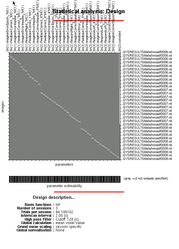
%Estimating the GLM can take some time, particularly if you have a lot of betas. If you just want to specify your
%design matrix so that you can assess it for singularities, turn this to 0.
%If you wish to do it later, estimating the GLM through the GUI is very
%quick.
ESTIMATE_GLM = 1;


%%%-----------------------------------------------------%%%


%For each subject, create timing files and jobs structure
for subject = subjects
    
    %See whether output directory exists; if it doesn't, create it
    outputDir = [rootDir num2str(subject) spmDir];
    
    if ~exist(outputDir)
        mkdir(outputDir)
    end
     
    %---Navigate to timing directory and create .mat files for each run---%
    cd([rootDir timingDir]);
    
    fid = fopen([num2str(subject) timingSuffix], 'rt');
    T = textscan(fid, '%f %s %f %f', 'HeaderLines', 1); %Columns should be 1)Run, 2)Regressor Name, 3) Onset Time (in seconds, relative to start of each run), and 4)Duration, in seconds
    fclose(fid);
    
    clear runs nameList names onsets durations sizeOnsets %Remove these variables if left over from previous analysis
    
    runs = unique(T{1});

    %Begin creating jobs structure
    jobs{1}.stats{1}.fmri_spec.dir = cellstr(outputDir);
    jobs{1}.stats{1}.fmri_spec.timing.units = 'secs';
    jobs{1}.stats{1}.fmri_spec.timing.RT = TR;
    jobs{1}.stats{1}.fmri_spec.timing.fmri_t = 16;
    jobs{1}.stats{1}.fmri_spec.timing.fmri_t0 = 1;

    %Create multiple conditions .mat file for each run
    for runIdx = 1:size(runs, 1)
            nameList = unique(T{2});
            names = nameList';
            onsets = cell(1, size(nameList,1));
            durations = cell(1, size(nameList,1));
            sizeOnsets = size(T{3}, 1);
        for nameIdx = 1:size(nameList,1)
            for idx = 1:sizeOnsets
                if isequal(T{2}{idx}, nameList{nameIdx}) && T{1}(idx) == runIdx
                    onsets{nameIdx} = double([onsets{nameIdx} T{3}(idx)]);
                    durations{nameIdx} = double([durations{nameIdx} T{4}(idx)]);
                end
            end
            onsets{nameIdx} = (onsets{nameIdx} - (TR*disacqs)); %Adjust timing for discarded acquisitions
        end

        save ([matPrefix '_' num2str(subject) '_' num2str(runIdx)], 'names', 'onsets', 'durations')
        
        %Grab frames for each run using spm_select, and fill in session
        %information within jobs structure
        files = spm_select('ExtFPList', [rootDir num2str(subject) dataDir], ['^' funcs{runIdx}], 1:numScans);

        jobs{1}.stats{1}.fmri_spec.sess(runIdx).scans = cellstr(files);
        jobs{1}.stats{1}.fmri_spec.sess(runIdx).cond = struct('name', {}, 'onset', {}, 'duration', {}, 'tmod', {}, 'pmod', {});
        jobs{1}.stats{1}.fmri_spec.sess(runIdx).multi = cellstr([outputDir matPrefix '_' num2str(subject) '_' num2str(runIdx) '.mat']);
        jobs{1}.stats{1}.fmri_spec.sess(runIdx).regress = struct('name', {}, 'val', {});
        jobs{1}.stats{1}.fmri_spec.sess(runIdx).multi_reg = {''};
        jobs{1}.stats{1}.fmri_spec.sess(runIdx).hpf = 128;
        
                
    end
    
    movefile([matPrefix '_' num2str(subject) '_*.mat'], outputDir)
    
    %Fill in the rest of the jobs fields
    jobs{1}.stats{1}.fmri_spec.fact = struct('name', {}, 'levels', {});
    jobs{1}.stats{1}.fmri_spec.bases.hrf = struct('derivs', [0 0]);
    jobs{1}.stats{1}.fmri_spec.volt = 1;
    jobs{1}.stats{1}.fmri_spec.global = 'None';
    jobs{1}.stats{1}.fmri_spec.mask = {''};
    jobs{1}.stats{1}.fmri_spec.cvi = 'AR(1)';
    
    %Navigate to output directory, specify and estimate GLM
    cd(outputDir);
    spm_jobman('run', jobs)
    
    if ESTIMATE_GLM == 1
        load SPM;
        spm_spm(SPM);
    end
    
end

%Uncomment the following line if you want to debug
%keyboard