Those who are the youngest children in the family are keenly aware of the disadvantages of being last in the pecking order; the quality of toys, clothes, and nutrition is often best for the eldest children in the family, and gradually tapers off as you reach the last kids, who are usually left with what are called, in parent euphemisms, "hand-me-downs."
In reality, these are things that should have been discarded several years ago due to being broken, unsafe, containing asbestos, or clearly being overused, such as pairs of underwear that have several holes in them so large that you're unsure of where exactly your legs go.
In SPM land, a similar thing happens to parametric modulators, with later modulators getting the dregs of the variance not wanted by the first modulators. Think of variance as toys and cake, and parametric modulators as children; everybody wants the most variance, but only the first modulators get the lion's share of it; the last modulators get whatever wasn't given to the first modulators.
The reason this happens is because when GLMs are set up, SPM uses a command, spm_orth, to orthogonalize the modulators. The first modulator is essentially untouched, but all other modulators coming after it are orthogonalized with respect to the first; and this proceeds in a stepwise function, with the second modulator getting whatever was unassigned to the first, the third getting whatever was unassigned to the second, and so on.
(You can see this for yourself by doing a couple of quick simulations in Matlab. Type x1=rand(10,1), and x2=rand(10,1), and then combine the two into a matrix with xMat = [x1 x2]. Type spm_orth(xMat), and notice that the first column is unchanged, while the second is greatly altered. You can then flip it around by creating another matrix, xMatRev = [x2 x1], and using spm_orth again to see what effect this change has.)
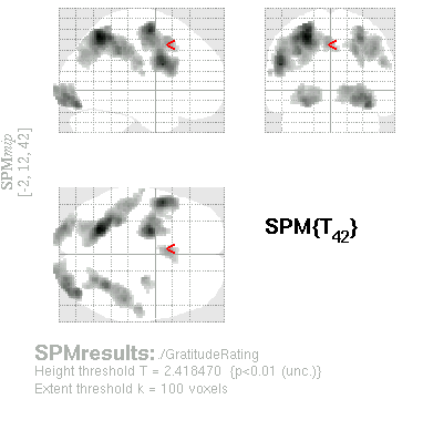
Be aware of this, as this can dramatically alter your results depending on how your modulators were ordered. (If they were completely orthogonal by design, then the spm_orth command should have virtually no impact; but this scenario is rare.) This came to my attention when looking at a contrast of a parametric modulator, which was one of three assigned to a main regressor. In one GLM, the modulator was last, and correspondingly explained almost no variance in the data; while in another GLM, the modulator was first, and loaded on much more of the brain. The following two figures show the difference, using exactly the same contrast and correction threshold, but simply reversing the order of the modulators:
In reality, these are things that should have been discarded several years ago due to being broken, unsafe, containing asbestos, or clearly being overused, such as pairs of underwear that have several holes in them so large that you're unsure of where exactly your legs go.
In SPM land, a similar thing happens to parametric modulators, with later modulators getting the dregs of the variance not wanted by the first modulators. Think of variance as toys and cake, and parametric modulators as children; everybody wants the most variance, but only the first modulators get the lion's share of it; the last modulators get whatever wasn't given to the first modulators.
The reason this happens is because when GLMs are set up, SPM uses a command, spm_orth, to orthogonalize the modulators. The first modulator is essentially untouched, but all other modulators coming after it are orthogonalized with respect to the first; and this proceeds in a stepwise function, with the second modulator getting whatever was unassigned to the first, the third getting whatever was unassigned to the second, and so on.
(You can see this for yourself by doing a couple of quick simulations in Matlab. Type x1=rand(10,1), and x2=rand(10,1), and then combine the two into a matrix with xMat = [x1 x2]. Type spm_orth(xMat), and notice that the first column is unchanged, while the second is greatly altered. You can then flip it around by creating another matrix, xMatRev = [x2 x1], and using spm_orth again to see what effect this change has.)
Be aware of this, as this can dramatically alter your results depending on how your modulators were ordered. (If they were completely orthogonal by design, then the spm_orth command should have virtually no impact; but this scenario is rare.) This came to my attention when looking at a contrast of a parametric modulator, which was one of three assigned to a main regressor. In one GLM, the modulator was last, and correspondingly explained almost no variance in the data; while in another GLM, the modulator was first, and loaded on much more of the brain. The following two figures show the difference, using exactly the same contrast and correction threshold, but simply reversing the order of the modulators:
 |
| Results window when parametric modulator was the last one in order. |
 |
| Results window when parametric modulator was the first one in order. |
This can be dealt with in a couple of ways:
- Comment out the spm_orth call in two scripts used in setting up the GLM: line 229 in spm_get_ons.m, and lines 285-287 in spm_fMRI_design.m. However, this might affect people who actually do want the orthogonalization on, and also this increases the probability that you will screw something up. Also note that doing this means that the modulators will not get de-meaned when entered into the GLM.
- Create your own modulators by de-meaning the regressor, inserting your value at the TR where the modulator occurred, then convolving this with an HRF (usually the one in SPM.xBF.bf). If needed, downsample the output to match the original TR.
It is well to be aware of all this, not only for your own contrasts, but to see how this is done in other papers. I recall reading one a long time ago - I can't remember the name - where several different models were used, in particular different models where the modulators were entered in different orders. Not surprisingly, the results were vastly different, although why this was the case wasn't clearly explained. Just something to keep in mind, as both a reader and a reviewer.
I should also point out that this orthogonalization does not occur in AFNI; the order of modulators has no influence on how they are estimated. A couple of simulations should help illustrate this:
 |
| Design matrices from AFNI with simulated data (one regressor, two parametric modulators.) Left: PM1 entered first, PM2 second. Right: Order reversed. The values are the same in both windows, just transposed to illustrate which one was first in the model. |
More information on the topic can be found here, and detailed instructions on how to construct your own modulators can be found on Tor Wager's lab website.