Andy's Brain Blog

That last tutorial on psychophysiological interactions - all thirteen minutes of it - may have been a little too much to digest in one sitting. However, you also don't understand what it's like to be in the zone, with the AFNI commands darting from my fingertips and the FMRI information tumbling uncontrollably from my lips; sometimes I get so excited that I accidentally spit a little when I talk, mispronounce words like "particularly," and am unable to string two coherent thoughts together. It's what my dating coach calls the vibe.

With that in mind, I'd like to provide some more supporting commentary. Think of it as supplementary material - that everybody reads!

Psychophysiological interactions (PPIs) are correlations that change depending on a given condition, just as in statistics. (The concept is identical, actually.) For example: Will a drug affect your nervous system differently from a placebo depending on whether you have been drinking or not? Does the effectiveness of Old Spice Nocturnal Creatures Scent compared to Dr. Will Brown's Nutty Time Special Attar (tm) depend on whether your haberdasher is Saks Fifth Avenue, or flophouse? Does the transcendental experience of devouring jar after jar of Nutella depend on whether you are alone, or noshing on it with friends? (Answer: As long as there's enough to go around, let the good times roll, baby!)

So much for the interaction part, but what about this psychophysiological thing? The "psychophysiological" term is composed of two parts, namely - and I'm not trying to insult your intelligence here - a psychological component and a physiological component. The "psychological" part of a PPI refers to which condition your participant was exposed to; perhaps the condition where she was instructed to imagine a warm, fun, exciting environment, such as reading Andy's Brain Blog with all of her sorority sisters during a pajama party on a Saturday night and trying to figure out what, exactly, makes that guy tick. Every time she imagines this, we code it with a 1; every time she imagines a contrasting condition, such as reading some other blog, we code that with a -1. And everything else gets coded as a 0.

Here are pictures to make this more concrete:

Figure 1: Sorority girls reading Andy's Brain Blog (aka Condition 1)

Figure 2: AvsBcoding with 1's, -1's, and 0's

The physiological component, on the other hand, simply refers to the underlying neural activity. Remember, however, that what we see in a typical FMRI timeseries isn't the actual neural activity; it's neural activity that has been smeared (i.e., convolved) with the hemodynamic response function, or HRF. To convert this back to the neural timeseries, we de-smear (i.e., deconvolve) the timeseries by removing the HRF - similar to a Fourier analysis if you have done one of those. (You have? NERD!)

To summarize: we assume that the observed timeseries is a convolution of the underlying neural activity with the HRF. Using NA for neural activity, HRF for the gamma response function, and (x) for the Kroenecker product, symbolically this looks like:

TimeSeries = NA (x) HRF

To isolate the NA part of the equation, we extract the TimeSeries from a contrast or some anatomically defined region, either using the AFNI Clusterize GUI and selecting the concatenated functional runs as an Auxiliary TimeSeries, or through a command such as 3dmaskave or 3dmaskdump. (In either case, make sure that the text file is one column, not one row; if it is one row, use 1dtranspose to fix it.) Let's call this ideal time series Seed_ts.1D.

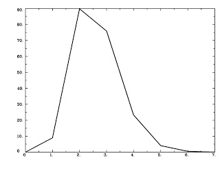
Next, we generate an HRF using the waver command and shuffle it into a text file:

waver -dt [TR] -GAM -inline 1@1 > GammaHR.1D

Check this step using 1dplot:

1dplot GammaHR.1D

And you should see something like this:

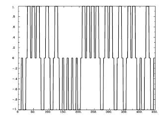
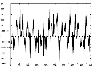
Now that we have both our TimeSeries and our HRF, we can calculate NA, the underlying neural activity, using 3dTfitter (the -Faltung option, by the way, is German for "deconvolution"):

3dTfitter -RHS Seed_ts.1D -FALTUNG GammaHR.1D Seed_Neur 012 0

This will tease apart GammaHR.1, from the TimeSeries Seed_ts.1D, and store it in a file called Seed_Neur.1D. This should look similar to the ideal time course we generated in the first step, except now it is in "Neural time":

1dplot Seed_Neur.1D

Ausgezeichnet! All we have to do now is multiply this by the AvsBcoding we made before, and we will have our psychophysiological interaction!

1deval -a Seed_Neur.1D -b AvsBcoding.1D -expr 'a*b' -prefix Inter_neu.1D

This will generate a file, Inter_neu.1D, that is our interaction at the neural level:

1dplot Inter_neu.1D

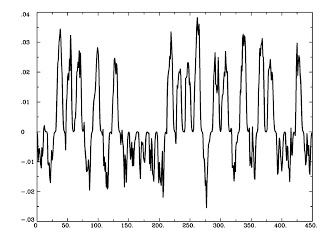
And, finally, we take it back into "BOLD time" by convolving this timeseries with the canonical HRF:

waver -dt 2 -GAM -input Inter_neu.1D -numout [numTRs] > Inter_ts.1D

1dplot Inter_ts.1D

Let's pause and review what we've done so far:

First, we extracted a timeseries from a voxel or group of voxels somewhere in the brain, either defined by a contrast or an anatomical region (there are several other ways to do this, of course; these are just the two most popular);
We then created a list of 1's, -1's, and 0's for our condition, contrasting condition, and all the other stuff, with one number for each TR;
Next, we created a Gamma basis function using the waver command, simulating the canonical HRF;
We used 3dTfitter to decouple the HRF from the timeseries, moving from "BOLD time" to "Neural time";
We created our psychophysiological interaction by multiplying our AvsBcoding by the Neural TimeSeries; and
Convolved this interaction with the HRF in order to move back to "BOLD time".

Our last step is to enter this interaction and the region's timeseries into our model. Since we are entering this into the model directly as is, and since we are not convolving it with anything, we will use the -stim_file option. Also remember to not use the -stim_base option, which is usually paired with -stim_file; we are still estimating parameters for this regressor, not just including it in the baseline model.

Below, I have slightly modified the 3dDeconvolve script used in the AFNI_data6 directory. The only two lines that have been changed are the stim_file options for regressors 9 and 10:

#!/bin/tcsh

set subj = "FT"

# run the regression analysis
3dDeconvolve -input pb04.$subj.r*.scale+orig.HEAD                       \
    -polort 3                                                           \
    -num_stimts 10                                                       \
    -stim_times 1 stimuli/AV1_vis.txt 'BLOCK(20,1)'                     \
    -stim_label 1 Vrel                                                  \
    -stim_times 2 stimuli/AV2_aud.txt 'BLOCK(20,1)'                     \
    -stim_label 2 Arel                                                  \
    -stim_file 3 motion_demean.1D'[0]' -stim_base 3 -stim_label 3 roll \
    -stim_file 4 motion_demean.1D'[1]' -stim_base 4 -stim_label 4 pitch \
    -stim_file 5 motion_demean.1D'[2]' -stim_base 5 -stim_label 5 yaw   \
    -stim_file 6 motion_demean.1D'[3]' -stim_base 6 -stim_label 6 dS    \
    -stim_file 7 motion_demean.1D'[4]' -stim_base 7 -stim_label 7 dL    \
    -stim_file 8 motion_demean.1D'[5]' -stim_base 8 -stim_label 8 dP    \
    -stim_file 9 Seed_ts.1D -stim_label 9 Seed_ts    \
    -stim_file 10 Inter_ts.1D -stim_label 10 Inter_ts    \
    -gltsym 'SYM: Vrel -Arel' -x1D X.xmat.1D -tout -xjpeg X.jpg                             \
    -bucket stats_Inter.$subj -rout

This will generate a beta weights for the Interaction term, which can then be taken to a group-level analysis using your command of choice. You can also do this with the R-values, but be aware that 3dDeconvolve will generate R-squared values; you will need to take the square root of these and then apply a Fisher's R-to-Z transform before you do a group analysis. Because of the extra steps involved, and because interpreting beta coefficients is much more straightforward, I recommend sticking with the beta weights.

Unless you're a real man like my dating coach, who recommends alpha weights.

This subject was brought to my attention by a colleague who wanted to know whether parametric modulation or duration modulation was a better way to account for RT effects. While it can depend on the question you are trying to answer, often duration modulation (referred to here as a "variable epoch model") works best. The following highlights the different approaches for modeling trials which involve a period of decision-making or an interval between presentation of a stimulus and the resulting response.

Over the past few years there has been a renewed interest in modeling duration in fMRI data. In particular, a methods paper by Grinband and colleagues (2008) compared the effects of modeling the duration of a trial - as measured by its reaction time (RT) - against models which used RT as a parametric modulator and against models which did not use RT at all. The argument against using RT-modulated regressors was that, at short time intervals (i.e., less than four seconds), using an impulse function was a good approximation to the resulting BOLD signal (cf. Henson, 2003).

Figure depicting relationship between stimulus onset, BOLD response, and underlying neural activity. Red lines: activity associated with punctate responses (e.g., light flashed at the subject). Blue lines: Activity associated with trials of unequal duration (e.g., decision-making).

However, for a few investigators, such assumptions were not good enough. To see whether different models of RT led to noticeable differences in BOLD signal, Grinband et al (2008) examined four types of modeling:

Convolving the onset of a condition or response with the canonical HRF (constant impulse model);
Separately modeling both the main effect of the condition as well as a mean-centered parametric modulator - in this case RT (variable impulse model);
Binning each condition onset into a constant amount of time (e.g., 2 seconds) and convolving with the canonical HRF (constant epoch model); and
Modeling each event as a boxcar function equal to the length of the subject's RT (variable epoch model).

Graphical summary of models from Grinband et al (2008). Top: Duration of cognitive process as indexed by reaction time. Constant Impulse: Onset of each event treated as a punctate response. Constant Epoch: Onset of each event convolved with boxcar function of constant duration. Variable Impulse: Punctate response functions modulated by mean-centered parameter (here, RT). Variable Epoch: Each event modeled by boxcar of duration equal to that event's RT.

Each of these models was then compared using data from a decision-making task in which subjects determined whether a line was long or short. If this sounds uninteresting to you, you have obviously never done a psychology experiment before.

The authors found that the variable epoch model - in other words, convolving each event with a boxcar equal to the length of the subject's RT for that trial - captured more of the variability in the BOLD response, in addition to reducing false positives as compared to the other models. The variable epoch model also dramatically increased sexual drive and led to an unslakeable thirst for mindless violence. Therefore, these simulations suggest that for tasks requiring time - such as decision-making tasks - convolution with boxcar regressors is a more faithful representation of the underlying neuronal dynamics (cf. the drift-diffusion model of Ratcliff & McKoon, 2008). The following figures highlight the differences between the impulse and epoch models:

Comparison of impulse models and epoch models as depicted in Grinband et al (2008). A) For impulse models, the shape remains constant while the amplitude varies; for epoch models, increasing the duration of a trial leads to changes in both shape and amplitude. B) Under the impulse model, increasing the duration of a stimulus or cognitive process (as measured by RT) leads to a reduction in explained variance.

Figure from Grinband et al (2008) showing differential effects of stimulus intensity and stimulus duration. Left: Increasing stimulus intensity has no effect on the time to peak of the BOLD response. Right: Increasing stimulus duration (or the duration of the cognitive process) leads to a linear increase in the time for the BOLD response to peak.

One caveat: note well that both parametric modulation and convolution with boxcar functions will account for RT-related effects in your data; and although the Grinband simulations establish the supremacy of boxcar functions, there may be occasions that warrant parametric modulation. For example, one may be interested in the differences of RT modulation for certain trial types as compared to others; and the regressors generated by parametric modulation will allow the researcher to test them against each other directly.