Duration Modulation in AFNI

Modulating signal by duration - usually reaction time (RT) - is increasingly common in fMRI data analysis, particularly in light of recent studies examining how partialing out RT can reduce or even eliminate effects in certain regions of the brain (e.g., anterior cingulate; see Grinband et al, 2010; Yarkoni et al, 2009). In light of these findings, it appears as though parametrically modulating regressors by RT, or the duration of a given condition, is an important factor in any analysis where this data is available.

When performing this type of analysis, therefore, it is important to know how your analysis software processes duration modulation data. With AFNI, the default behavior of their duration modulation basis function (dmBLOCK) used to scale everything to 1, no matter how long the trial lasted. This may be useful for comparison to other conditions which have also been scaled the same way, but is not an appropriate assumption for conditions lasting only a couple of seconds or less. The BOLD response tends to saturate over time when exposed to the same stimulation for an extended period (e.g., block designs repeatedly presenting visual or auditory stimulation), and so it is reasonable to assume that trials lasting only a few hundred milliseconds will have less of a ramping up effect in the BOLD response than trials lasting for several seconds.

The following simulations were generated with AFNI's 3dDeconvolve using a variation of the following command:

3dDeconvolve -nodata 350 1 -polort -1 -num_stimts 1 -stim_times_AM1 q.1D 'dmBLOCK' -x1D stdout: | 1dplot -stdin -thick -thick

Where the file "q.1D" contains the following:

10:1 40:2 70:3 100:4 130:5 160:6 190:7 220:8 250:9 280:30

In AFNI syntax, this means that event 1 started 10 seconds into the experiment, with a duration of 1 second; event 2 started 40 seconds into the experiment with a duration of 2 seconds, and so on.

The 3dDeconvolve command above is a good way to generate simulation data, through the "-nodata" option which tells 3dDeconvolve that there is no functional data to process. The command tells 3dDeconvolve to use dmBLOCK as a basis function, convolving each event with a boxcar function the length of the specified duration.

Running this command as is generates the following graph:

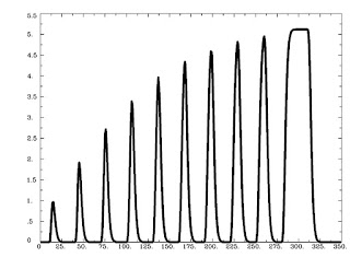
As is expected, trials that are shorter are scaled less, while trials lasting longer are scaled more, with a saturation effect occurring around 8-9 seconds.

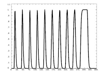
Running 3dDeconvolve with a basis function scaling the signal change in each to 1 is done with the following:

3dDeconvolve -nodata 350 1 -polort -1 -num_stimts 1 -stim_times_AM1 q.1D 'dmBLOCK(1)' -x1D stdout: | 1dplot -stdin -thick -thick

And generates the following output:

Likewise, the ceiling on the basis function can be set to any arbitrary number, e.g.:

3dDeconvolve -nodata 350 1 -polort -1 -num_stimts 1 -stim_times_AM1 q.1D 'dmBLOCK(10)' -x1D stdout: | 1dplot -stdin -thick -thick

However, the default behavior of AFNI is to scale events differently based on different duration (and functions identically to the basis function dmBLOCK(0)). This type of "tophat" function makes sense, because unlimited signal increase as duration also increases would lead to more and more bloodflow to the brain, which, taken to its logical conclusion, would mean that if you showed someone flashing checkerboards for half an hour straight their head would explode.

As always, it is important to look at your data to see how well your model fits the timecourse of activity in certain areas. While it is reasonable to think that dmBLOCK(0) is the most appropriate basis function to use for duration-related trials, this may not always be the case.

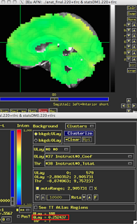
These last two figures show the same subject analyzed with both dmBLOCK(0) and dmBLOCK(1). The underlying beta values for each do not differ significantly, although there is some variability in how much they differ in distinct cortical areas, and small but consistent changes in variability can lead to relatively large effects at the second level.

The image on the left hasn't been masked, but the underlying beta estimates should be the same in either case.

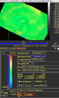
dmBLOCK(0)

dmBLOCK(1)

Karl Friston's Rules for Reviewing

This post was orphaned a while back when I was testing links to papers, but I figured I should go back and explain what I was doing. This is a link to Friston's recent Neuroimage paper giving advice to young reviewers for how to reject any paper, regardless of how scientifically and statistically sound it is. His tone is purposely ironic, although he takes a more serious turn at the end in explaining why these rejection criteria are ridiculous.

The link to Friston's paper can be found here.

SUMA Demo

I've posted a demo of AFNI's surface mapper program, SUMA, over here on my screencast account. Specifically, I talk about how to map volumetric results generated in any fMRI software package (e.g., AFNI, FSL, SPM, BrainVoyager) onto a template surface provided by SUMA.

In this demo, I take second-level results generated in SPM and map them onto a template MNI surface, the N27 brain. All that is needed for doing this is a results dataset, a template underlay anatomical brain to visualize results on (here I use the MNI_caez_N27 brain provided in the AFNI binaries directory under ~/abin), and a folder called suma_mni that contains the .spec files for mapping onto the N27 brain. The suma_mni folder is available for download at Ziad Saad's website here. Just download it to the same directory, and you are good to go.

SPM 2nd-level results mapped onto template surface using AFNI / SUMA

I've outlined the steps in a word document, Volumetric_SUMA.docx, which is available at my website. Please send me any feedback if any of the steps are unclear.

Although this is an incredibly easy way to make great-looking figures, at the same time I would not recommend doing any ROI stats on the results mapped onto a surface using these steps. This is because it is essentially a rough interpolation of which voxel corresponds to which node; if you want to do surface ROI analyses, do all of your preprocessing and statistics on the surface (I may write up a demo of how to do this soon).

Python SUITE: AFNI_Tools.gz

This is an update from my earlier post about the Python program convertDICOM2AFNI.py; now it is a folder containing a few programs that interact with each other. The rationale was to give the original dicom conversion script a wrapper that can change directory (since I am currently unable to do this from the python interpreter invoked by the Unix shell). All the user needs to do is download the file AFNI_Tools.gz into their home directory, unzip it using "tar -zxvf AFNI_Tools.gz" into your experimental directory, and run it using the command "tcsh convertRaw2AFNI.sh". The user will be prompted for a list of subject IDs, the name of the experimental directory, and will then run the script convertDICOM2AFNI.py inside the raw fMRI data folder for each subject. This in turn will prompt the user for study-specific info, such as number of slices, number of TRs, and so on. Currently, there is no way to account for runs with different numbers of TRs; I may add this function in the future.

A short screencast demo of the suite is available at www.screencast.com/users/Andrew.Jahn/folders/Jahn_Tools (you may need to go full-screen mode in order to see what I'm typing on the command line). What I did not mention in the demo is the subfolder "Paths" within the AFNI_Tools folder. It contains two text files, groupDir.txt and dataDir.txt. groupDir.txt contains the path to the experimental directory, while dataDir.txt contains the path to the output directory that you want for each subject; these should be modified when you download the suite. I've included some documentation that I hope is enough to get people started.

In addition, after converting the raw scanner files to both AFNI and NIFTI format, the program will drive AFNI directly from the command line and allow the user to interactively scroll through each functional dataset. For example, the first run of functional data will be displayed and a video of its timecourse will start playing; this is a good way to visually check for any scanner artifacts or excessive head motion, and deciding what to do with it. You can then hit enter in the terminal window that generated AFNI, and it will skip to the next functional run of data, and so on. The idea is to make it easy to do a first-pass analysis on your raw data and see whether anything is completely out of line.

As always, please send me feedback if you have actually used the program, and what you think about it.


=====================
P.S. Photos from the AFNI bootcamp are now up. I now have photographic evidence that I was at the National Institutes of Health, and not somewhere else, like Aruba.

AFNI Bootcamp / Proof that I was not in Aruba

Ye Good Olde Days

I've uploaded my powerpoint presentation about what I learned at the AFNI bootcamp; for the slides titled "AFNI Demo", "SUMA Demo", and so on, you will have to use your imagination.

The point of the presentation is that staying close to your data - analyzing it, looking at it, and making decision about what to do with it - are what we are trained to do as cognitive neuroscientists (really, any scientific discipline). The reason I find AFNI to be superior is that it allows the user to do this in a relatively easy way. The only roadblocks are getting acquainted with Unix and shell programming, and also taking the time to get a feel for what looks normal, and what looks potentially troublesome.

Back in the good old days (ca. 2007-2008) we would simply make our scripts from scratch, looking through fMRI textbooks and making judgments about what processing step should go where, and then looking up the relevant commands and options to make that step work. Something would inevitably break, and if you were like me you would spend days or weeks trying to fix it. To make matters worse, if you asked for help from an outside source (such as the message boards), nobody had any idea what you were doing.

The recent scripts containing the "uber" prefix - such as "uber_subject.py", "uber_ttest.py", and so on - have mitigated this problem considerably, generating streamlined scripts that are more or less uniform across users, and therefore easier to compare and troubleshoot. Of course, you still need to go into the generated script and make some modifications here and there, but everything is pretty much in place. It will still suggest that you check each intermediate step, but that becomes easier to ignore once you have a higher-level interface that takes care of all the minor details for you. Like everything else, there are tradeoffs.

Python Script: convertDICOM2AFNI.py

I've written my first (useful) python script, a small program called convertDICOM2AFNI.py, that looks for DICOM files from our scanner and converts them to AFNI format. Converting raw scanner data to AFNI format using the to3d command is light years (i.e., minutes) faster than SPM's DICOM import, or MRIcron's dcm2nii program. dcm2nii, in particular, usually gave me a bunch of other files that I was never interested in and would convert everything in my raw DICOM folder, even though there were only a few runs that I was interested in looking at. It would also introduce some weird temporal interpolations into the data, modifying the header information to make it appear as though the volumes were slice-time corrected even though they actually were not.

In order to get around this problem, I may add an option to the script which converts to AFNI, and then converts to nifti format using 3dAFNI2NIFTI (although I have no idea what might get lost in the translation; will need to do some testing here).

To use the script, do the following:

1) Create folder containing all raw DICOM files generated from your experiment
2) Write down which session numbers correspond with which functional and anatomical runs (remember: pencil & paper are your friends)
3) Run the script from the raw DICOM directory using the command "python convertDICOM2AFNI.py"

It will ask you a series of questions about which session numbers are your functional runs, and then which session is your anatomical run. If you run the command without defaults (i.e., without using the "-d") flag, it will also ask you the number of slices in the z-direction, the number of TRs, and the length of each TR in milliseconds.

In the future, I plan to have the program automatically read in a defaults file that specifies all of these arguments automatically. However, that also assumes that the user is organized (which I am not). Also, as of this writing, it assumes that the z-slices alternate positively in the z-direction; if this is not true for you, you may need to change the script yourself.

The script is available for download over at my webpage (http://mypage.iu.edu/~ajahn) under "Python Scripts". The actual location of the scripts I write will probably change as I become more organized.


I plan to begin writing a suite of Python programs that I find useful for interacting with both SPM and AFNI data, eventually working up to a GUI sometime in the far future. For now, it will assume a degree of command line proficiency and that you can probably figure things out if the script does not perfectly fit your needs.


===============================

Due to high demand from the Scottish population at IU, a screencast will soon be up detailing how to interpolate volumetric data onto a template surface.

New Webpage

I have a new webpage over on the IU servers, which contains a professional-looking picture of me and links to stuff that may be useful. Some of the resources I have posted are relatively specific to my lab, so take that into consideration before using them. I am not responsible for whatever happens if you do use them.

AFNI Bootcamp: Day 4

Finally, I’ve made it to the last day of bootcamp. Got an AFNI pen to prove that I was here, and pictures of the workshop should be available shortly, since I’m assuming everyone must be curious to know what it looked like (I would be).

Gang opened with a presentation on the AFNI tools available for the primary types of connectivity: functional connectivity and effective connectivity. Functional connectivity is a slightly misleading term in my opinion, since you are simply looking at correlations between regions based on a seed-voxel timeseries. The correlation we claim to be looking at is merely a goodness of fit of the timeseries of one voxel with another, and from there we state whether these regions are somehow talking to each other or not, although that is a nebulous term. Much safer would be to go with a term like timeseries correlation analysis, since that is more descriptive of what is actually going on. As for effective connectivity and other types of intra and inter-voxel correlations such as structural equation modeling, I have not had as much experience in those areas, and will not touch on them right now. When I get to those sometime down the line, I will discuss those in more detail, and whether and when they appear to be useful.

The remained of the day was a SUMA demo from Ziad, showcasing how easy it is to visualize surface activity using their surface mapping program. SUMA is, in my experience, much faster and easier to manipulate than FreeSurfer, and, notwithstanding a few technical hurdles, is simple to use when interfacing with volumetric data. Also demonstrated was AFNI’s InstaCorr tool, which allows for instantaneous visualization of functional connectivity throughout the entire brain. One simply sets a voxel as a seed region, and can see how it correlates with every other voxel in the brain. The most interesting (and fun) feature of this tool is the ability to simply hold down the control and shift keys, and then drag the mouse cursor around to see the functional connectivity maps update in less time than it takes to refresh the monitor. This can be done on the surface maps as well. Although I still have the same reservations about resting state data as mentioned previously, this appears to be an excellent method for visualizing these experiments.

Beyond that, I took the opportunity to get in some additional face time with each of the AFNI members, and had a conversation with Daniel about how to examine registration between anatomical and epi datasets. By adding the –AddEdge option to the alignment part of the script (such as align_epi_anat.py), an additional folder named “AddEdge” is created with the anatomical and EPI datasets both before and after registration. Contours of the gyri and sulci are also shown, as well as any overlap between the two after registration. Apparently, the functional data I showed him wasn’t particularly defined (although we were acquiring at 3.5x3.5x3.75), the registration was still OK. One method for improving it may be to use scans acquired pre-steady-state, since those have been spatial contrast than the scans that are acquired during the experiment.

Before I left, I asked Bob about using grey matter masks for smoothing. The rationale for smoothing within a grey matter mask is to avoid smoothing in air and other stuff that we don’t care about (e.g., CSF, ventricles, bone), and as a result improve SNR relative to traditional smoothing methods that take place over the entire brain. However, Bob brought up the point that smoothing within GM on an individual subject basis can introduce biases into the group analysis, since not every subject experiences the same smoothing in the same voxel location. When we smooth, for example, after normalizing to a standardized space, all of the brains fit within the magic Talairach box, and so everything within the bounding box receives the same smoothing kernel. However, since each subject’s grey matter boundaries are stereotyped, we may be smoothing in different areas for each subject; in fact, it is guaranteed to happen. To alleviate this, one could either create a group grey matter mask and use that for smoothing, or take both the white and grey matter segmentation maps from FreeSurfer and, combining them, smooth across a whole brain mask that leaves out non-brain related areas, such as ventricles. I will have to think more about this and try a couple of approaches before deciding on what is feasible, and whether it makes that big of a difference or not.

That’s about it from the bootcamp. It has been an intense four days, but I have enjoyed it immensely, and I plan to continue using AFNI in the future, at least for double-checking the work that goes on in my lab. I’ll be experimenting more in the near future and posting figures of my results, as well as screencasts, when I find the time to pick those up again. For now, it’s onto CNS at Chicago.

AFNI Bootcamp: Day 3

Today, Bob began with an explanation for how AFNI’s amplitude modulation (cf. SPM’s parametric modulation) differs from other software approaches. For one, not only are the estimates for each parametric modulation computed, but so is the estimate of the beta itself. This leads to estimates of what variance can be explained by the parametric modulators, above and beyond the beta itself. Then, the beta estimates for those parametric modulators can be carried to the second level, just like any other parameter estimate.

To give a concrete example, take an experiment that presents the subject with a gamble that varies on three specific dimensions: probability of win, magnitude of win, and the variance of the gamble. Let us say that the onset of the gamble occurred at 42 seconds into the run, and that the dimensions were 0.7, 10, and 23. In this case, the onset time of the gamble would be parametrically modulated by these dimensions, and would be represented in a timing file as 42*0.7,10,23.  [Insert AM_Example.jpg here]. Notice that the resulting parametric modulators are mean-centered, here resulting in negative values for probability and variance. The purpose of the amplitude modulation is to see what proportion of the variance in the BOLD response is due to these additional variables driving the amplitude of the BOLD signal; if it is a particularly good fit, then the resulting t-statistic for that beta weight will be relatively high.

Regarding this, 3dREMLfit was mentioned yet again, as Bob pointed out how it takes into account both the beta estimate and the variance surrounding that estimate (i.e., the beta estimate’s associated t-statistic). A high beta estimate does not necessarily imply a high t-statistic, and vice versa, which is why it would make sense to include this information at the group level. However, none of the AFNI developer’s that I talked to definitively stated that 3dMEMA or the least-squares method was preferable; that is entirely up to the user. I examined this with my own data, looking at a contrast of two regressors at the 2^nd-level using both OLSQ and 3dMEMA. As the resulting pictures show, both methods show patterns of activation in the rostral ACC (similar to what I was getting with SPM), although 3dMEMA produces an activation map that passes cluster correction, while OLSQ does not. Which should you use? I don’t know. I suppose you can try both, and whatever gives you the answer that you want, you should use. If you use 3dMEMA and it doesn’t give you the result that you want, you can just claim that it’s too unreliable to be used just yet, and so make yourself feel better about using a least-squares approach.

After a short break, Ziad discussed AFNI’s way of dealing with resting state data via a program called RETROICOR. I have no idea what that stands for, but it accounts for heart rate and respiration variability for each subject, which is critically important when interpreting a resting state dataset. Because the relationship between physiological noise –especially heart rate – and the BOLD signal is poorly understood, it is reasonable to covary this activation out, in order to be able to claim that what you are looking at is true differences in neural activation between conditions or groups or whatever you are investigating (although using the term “neural activation” is a bit of a stretch here). Apparently this is not done that often, and neither is accounting for motion, which can be a huge confound as well.  All of the confounds listed above can lead to small effect sizes biased in a certain direction, but can do so consistently, leading to significant activation at the group level that has nothing to do with the participant’s true resting state (although again, the term “resting state” is a bit of a stretch, since you have no idea what the participant is doing, and no tasks to regress to explain the timeseries data). In any case, this is an area I know very little about, but the potential pitfalls seem serious enough to warrant staying away from this unless I have a really good reason for doing it.

AFNI Bootcamp: Day 2

Today was a walkthrough of the AFNI interface, and a tutorial for how to view timeseries data and model fits. Daniel started off with a showcase of AFNI’s ability to graph timeseries data for each stage of preprocessing, and how it changes as a result of each step. For example, after scaling the raw MR signal to a percentage, the values at each TR in the timeseries graph begin to cluster around the value of 100. This is a totally arbitrary number, but allows one to make inferences about percent signal change, as opposed to simply parameter estimates. Since this percent signal change is done for each voxel, as opposed to grand mean scaling in SPM which divides each voxel’s value by the mean signal intensity across the entire brain, it becomes more reasonable to talk in terms of percent signal change at each voxel.

Another cool feature is the ability to overlay the model fits produced by 3dDeconvolve on top of the raw timeseries. This is especially useful when looking all over the brain to see how different voxels correlate with the model (although this may be easier to see with a block design as opposed to an event-related design). You can extract an ideal time series from the X matrix output by 3dDeconvolve by using 1dcat [X Matrix column] > [output 1D file], and then overlay one or more ideal timeseries by clicking on Graph -> 1dTrans -> Dataset#. (Insert picture of this here).

One issue that came up when Ziad was presenting, was the fact that using dmBLOCK as a basis function to convolve an onset with a boxcar function does not take individual scaling into account. That is, if one event lasts six seconds, and another lasts ten seconds, they will be scaled by the same amount, although in principal they should be different, as saturation has not been achieved yet. I asked if they would fix this, and they said that they would, soon. Fingers crossed!

Outside of the lectures, Bob introduced me to AlphaSim’s successor, ClustSim. For those who haven’t used it, AlphaSim calculates how many contiguous voxels at a you need at a specified uncorrected threshold in order to pass a corrected cluster threshold. That is, AlphaSim runs several thousand simulations of white noise, and calculates the extent of uncorrected voxels that would appear at different levels of chance. ClustSim does the same thing, except that it is much faster, and can calculate several different corrected thresholds simultaneously. The uber scripts call on ClustSim to make these calculations for the user, and then write this information into the header of the statistics datasets. You can see the corrected cluster thresholds for each cluster under the “Rpt” button of the statistics screen.

On a related note, ClustSim takes into account smoothing that was done by the scanner before any preprocessing. I had no idea this happened, but apparently the scanners are configured to introduced very low-level (e.g., 2mm) smoothing into each image as it is output. Because of this, the uber scripts estimate the average amount of smoothness across an entire subject in the x, y, and z directions, which are not always the same. Therefore, if you used a smoothing kernel of 4mm, your estimated smoothness may be closer to 6mm. This is the full width at half max that should be used when calculating cluster correction levels in AlphaSim or ClustSim. Another tidbit I learned is that Gaussian Random Fields (SPM’s method of calculating cluster correction) is “difficult” at smoothing kernels less than 10mm. I have no idea why, but Bob told me so, so I treat it as gospel. Also, by “difficult”, I mean that it has a hard time finding a true solution to the correct cluster correction level.

I found out that, in order to smooth within a mask such as grey matter, AFNI has a tool named 3dBlurInMask for that purpose. This needs to be called at the smoothing step, and replaces 3dmerge or 3dFWHMx, whichever you are using for smoothing. This sounds great in theory, since most of the time we are smoothing both across white matter and a bunch of other crap from outside the brain which we don’t care about. At least, I don’t care about it. The only drawback is that it suffers from the same problem as conventional smoothing, i.e. that there is no assurance of good overlap between subjects, and the resulting activation may not be where it was at the individual level. Still, I think it is worth trying out.

The last person I talked to was Gang Chen, the statistician. I asked him whether AFNI was going to implement a Bayesian inference application anytime soon, for parameter estimation. He told me that such an approach was unfeasible at the voxel level, as calculating HDIs are extremely computationally intensive (just think of how many chains, samples, thinning, etc, and then multiply that by tens of thousands of individual tests). Although I had heard that FSL uses a Bayesian approach, this isn’t really Bayesian; it is essentially the same as what 3dMEMA does, which is to weight high-variability parameter estimates less than high-precision parameter estimates. Apparently a true-blue Bayesian approach can be done (at the second level), but this can take up to several days. Still, it is something I would like to investigate more, and to compare results from AFNI to FSL’s Bayesian method, and see if there is any meaningful difference between the two.