K-Means Analysis with FMRI Data

Clustering, or finding subgroups of data, is an important technique in biostatistics, sociology, neuroscience, and dowsing, allowing one to condense what would be a series of complex interaction terms into a straightforward visualization of which observations tend to cluster together. The following graph, taken from the online Introduction to Statistical Learning in R (ISLR), shows this in a two-dimensional space with a random scattering of observations:


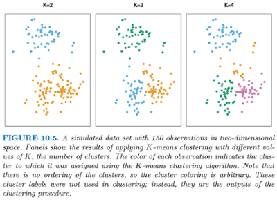
Different colors denote different groups, and the number of groups can be decided by the researcher before performing the k-means clustering algorithm. To visualize how these groups are being formed, imagine an "X" being drawn in the center of mass of each cluster; also known as a centroid, this can be thought of as exerting a gravitational pull on nearby data points - those closer to that centroid will "belong" to that cluster, while other data points will be classified as belonging to the other clusters they are closer to.

This can be applied to FMRI data, where several different columns of data extracted from an ROI, representing different regressors, can be assigned to different categories. If, for example, we are looking for only two distinct clusters and we have several different regressors, then a voxel showing high values for half of the regressors but low values for the other regressors may be assigned to cluster 1, while a voxel showing the opposite pattern would be assigned to cluster 2. The label itself is arbitrary, and is interpreted by the researcher.

To do this in Matlab, all you need is a matrix with data values from your regressors extracted from an ROI (or the whole brain, if you want to expand your search). This is then fed into the kmeans function, which takes as arguments the matrix and the number of clusters you wish to partition it into; for example, kmeans(your_matrix, 3).

This will return a vector of numbers classifying a particular row (i.e., a voxel) as belonging to one of the specified clusters. This vector can then be prefixed to a matrix of the x-, y-, and z-coordinates of your search space, and then written into an image for visualizing the results.

There are a couple of scripts to help out with this: One, createBlankNIFTI.m, which will erase a standardized space image (I suggest a mask output by SPM at its second level) and replace every voxel with zeros, and the other script, createNIFTI.m, will fill in those voxels with your cluster numbers. You should see something like the following (here, I am visualizing it in the AFNI viewer, since it automatically colors in different numbers):

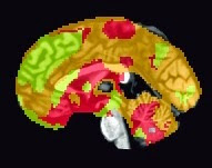
Sample k-means analysis with k=3 clusters.

The functions are pasted below, as well as a couple of explanatory videos.


function createBlankNIFTI(imageFile)

%Note: Make sure that the image is a copy, and retain the original

X = spm_read_vols(spm_vol(imageFile));
X(:,:,:) = 0;
spm_write_vol(spm_vol(imageFile), X);


=================================

function createNIFTI(imageFile, textFile)


hdr = spm_vol(imageFile);
img = spm_read_vols(hdr);

fid = fopen(textFile);
nrows = numel(cell2mat(textscan(fid,'%1c%*[^\n]')));
fclose(fid);

fid = 0;


for i = 1:nrows
    if fid == 0
        fid = fopen(textFile);
    end
    
    Z = fscanf(fid, '%g', 4);
    
    img(Z(2), Z(3), Z(4)) = Z(1);
    spm_write_vol(hdr, img);
end


Beta Series Analysis in SPM

The following is a script to run beta series analysis in SPM; which, conceptually, is identical to beta series analysis in AFNI, just made more complicated by the use of Matlab commands, many of which I would otherwise remain totally ignorant of.

Also, if you believe that I did this on my own, you are a scoundrel and a fool. Virtually all of the code is from my colleague Derek Nee, a postdoc who used to work in my lab and who remains my superior in all things, scientific and otherwise. He also once got me with the old "If you say gullible slowly, it sounds like orange" joke.

In any case, all that I did was repackage it into a function to be more accessible by people outside of our lab. You may see a couple snippets of code that are useful outside of just doing beta series analysis; for example, the spm_get_data command, which can be used for parameter extraction from the command line without using marsbar. Also note that the script assumes that each trial for a condition has been labeled separately with the regressor name followed by a "_" and then the occurrence of the trial. So, for example, if I were looking at 29 instances of pressing the left button, and the regressor name was LeftButtonPress, I would have LeftButtonPress_1, LeftButtonPress_2, LeftButtonPress_3...LeftButtonPress_29.

Obviously, this is very tedious to do by hand. The Multiple Conditions option through the SPM GUI for setting up 1st level analyses is indispensable; but to cover that is another tutorial, one that will probably cross over into our discussion of GLMs.


The script:

function DoBetaSeries(rootdir, subjects, spmdir, seedroi, Conds, MapNames)
% function BetaSeries(rootdir, subjects, spmdir, seedroi, Conds, MapNames)
% INPUT:
%  rootdir  - Path to where subjects are stored
%  subjects - List of subjects (can concatenate with brackets)
%  spmdir   - Path to folder containing SPM file
%  seedroi  - Absolute path to file containing ROI in NIFTI format
%  Conds    - List of conditions for beta series analysis
%  MapNames - Output for list of maps, one per Conds cell
%       
%   Example use:
%       BetaSeries('/data/study1/fmri/', [101 102 103],
%       'model/BetaSeriesDir/', '/data/study1/Masks/RightM1.nii',
%       {'TapLeft'}, {'TapLeft_RightM1'})
%
%       conditions to be averaged together should be placed together in a cell
%       separate correlation maps will be made for each cell
%       Conds = {'Incongruent' 'Congruent' {'Error' 'Late'}}; 
%
%       For MapNames, there should be one per Conds cell above
%       e.g., with the Conds above, MapNames = {'Incongruent_Map',
%       'Congruent_Map', 'Error_Late_Map'}
%
%       Once you have z-maps, these can be entered into a 2nd-level
%       1-sample t-test, or contrasts can be taken between z-maps and these
%       contrasts can be taken to a 1-sample t-test as well.
%
% 

if nargin < 5
 disp('Need rootdir, subjects, spmdir, seedroi, Conds, MapNames. See "help BetaSeries" for more information.')
    return
end


%Find XYZ coordinates of ROI
Y = spm_read_vols(spm_vol(seedroi),1);
indx = find(Y>0);
[x,y,z] = ind2sub(size(Y),indx);
XYZ = [x y z]';


%Find each occurrence of a trial for a given condition
%These will be stacked together in the Betas array
for i = 1:length(subjects)
    subj = num2str(subjects(i));
    disp(['Loading SPM for subject ' subj]);
    %Can change the following line of code to CD to the directory
    %containing your SPM file, if your directory structure is different
    cd([rootdir subj filesep spmdir]);
    load SPM;
    
    for cond = 1:length(Conds)
        Betas = [];
        currCond = Conds{cond};
        if ~iscell(currCond)
            currCond = {currCond};
        end
        for j = 1:length(SPM.Vbeta) 
            for k = 1:length(currCond)
                if ~isempty(strfind(SPM.Vbeta(j).descrip,[currCond{k} '_'])) 
                    Betas = strvcat(Betas,SPM.Vbeta(j).fname);
                end
            end
        end
              

    %Extract beta series time course from ROI
    %This will be correlated with every other voxel in the brain
    if ischar(Betas)
        P = spm_vol(Betas);
    end

    est = spm_get_data(P,XYZ);
    est = nanmean(est,2);


        %----Do beta series correlation between ROI and rest of brain---%

            MapName = MapNames{cond};
            disp(['Performing beta series correlation for ' MapName]);
            
            Vin = spm_vol(Betas);
            nimgo = size(Vin,1);
            nslices = Vin(1).dim(3);

            % create new header files
            Vout_r = Vin(1);   
            Vout_p = Vin(1);
            [pth,nm,xt] = fileparts(deblank(Vin(1).fname));
            Vout_r.fname = fullfile(pth,[MapNames{cond} '_r.img']);
            Vout_p.fname = fullfile(pth,[MapNames{cond} '_p.img']);

            Vout_r.descrip = ['correlation map'];
            Vout_p.descrip = ['p-value map'];

            Vout_r.dt(1) = 16;
            Vout_p.dt(1) = 16;

            Vout_r = spm_create_vol(Vout_r);
            Vout_p = spm_create_vol(Vout_p);

            % Set up large matrix for holding image info
            % Organization is time by voxels
            slices = zeros([Vin(1).dim(1:2) nimgo]);
            stack = zeros([nimgo Vin(1).dim(1)]);
            out_r = zeros(Vin(1).dim);
            out_p = zeros(Vin(1).dim);


            for i = 1:nslices
                B = spm_matrix([0 0 i]);
                %creates plane x time
                for j = 1:nimgo
                    slices(:,:,j) = spm_slice_vol(Vin(j),B,Vin(1).dim(1:2),1);
                end

                for j = 1:Vin(1).dim(2)
                    stack = reshape(slices(:,j,:),[Vin(1).dim(1) nimgo])';
                    [r p] = corr(stack,est);
                    out_r(:,j,i) = r;
                    out_p(:,j,i) = p;

                end

                Vout_r = spm_write_plane(Vout_r,out_r(:,:,i),i);
                Vout_p = spm_write_plane(Vout_p,out_p(:,:,i),i);

            end

                
            %Convert correlation maps to z-scores
            %NOTE: If uneven number of trials in conditions you are
            %comparing, leave out the "./(1/sqrt(n-3)" term in the zdata
            %variable assignment, as this can bias towards conditions which
            %have more trials
            
                disp(['Converting correlation maps for subject ' subj ', condition ' MapNames{cond} ' to z-scores'])
                P = [MapNames{cond} '_r.img'];
                n = size(Betas,1);
                Q = MapNames{cond};
                Vin = spm_vol([MapNames{cond} '_r.img']);

                % create new header files
                Vout = Vin;   

                [pth,nm,xt] = fileparts(deblank(Vin(1).fname));
                Vout.fname = fullfile(pth,[Q '_z.img']);

                Vout.descrip = ['z map'];

                Vout = spm_create_vol(Vout);

                data = spm_read_vols(Vin);
                zdata = atanh(data)./(1/sqrt(n-3));

                spm_write_vol(Vout,zdata);

    end
end


This can either be copied and pasted into a script, or downloaded as a .m file here.


Resting State Analysis, Part VII: The End

For the last part of the analysis, we are going to simply take all of the z-maps we have just created, and enter them into a second-level analysis across all subjects. To do this, first I suggest creating separate directories for the Autism and Control subjects, based on the phenotypic data provided by the KKI on the ABIDE website; once you have those, run uber_ttest.py to begin loading Z-maps from each subject into the corresponding category of Autism or Control.

Most of this is easier to see than to describe, so I've made a final tutorial video to show how this is all done. Hope it helps!


P.S. I've collated all of the past videos over the past week and a half into a playlist, which should make sorting through everything slightly easier:

AFNI's uber_subject.py


Back in the good old days, we would create our scripts ex nihilo; out of nothingness would we construct gigantic, Babel-esque scripts that nobody - to be honest, not even we - could understand. We would pore over FMRI textbooks and fumble around with commands and tools we thought were germane, only to have everything collapse all around us when it came time for execution. I remember with painful clarity the moment when I finally hit upon the idea of looping over subjects for each iteration of the script; I thought I was a creative genius.

Lawless, ruthless, and terrifying; those days were like the wild west. Nobody knew what the hell was going on; you might come across a block of analysis script posted by some group in Singapore, compare it to your own, and wonder how your two labs could ever come to the same conclusion about anything, given how radically different your scripts were. Your script would call for slice timing correction, followed by coregistration and normalization, while their script would call for a cup of chopped onions and a clove of chopped garlic. Then, slowly, you would realize that what you were looking at was a recipe for chicken cacciatore or something, and you would feel like an idiot. Overall, those days were not good.

Fortunately for us, these days we now have a script called uber_subject.py, which takes care of generating analysis scripts quickly and easily. AFNI script ex machina, as it were. If you have programs and binaries from the past couple of years or so (and there's no reason you shouldn't; if you haven't updated in a while, a quick '@update.afni.binaries -d', without the quotes, should do the trick), you will have uber_subject.py. If you type it from the command line - and your python libraries are current and functional (see here for a message board thread if you have trouble with this) - then a graphical user interface will pop up, prompting you to input parameters such as smoothing kernel size, number of regressors, relationship status, and so forth, until you have a completely idiosyncratic script to fit your needs. Overall it has worked very well for me so far, and word is that it will be integrated with an even higher level script called uber_script.py. I've had some issues getting it to work, so instead of trying to fix it, I have taken the path of least resistance and settled for uber_subject.py. You will be glad that you did as well.


Andy's Brain Blog Book Club: Lolita

The one non-scandalous image of Lolita I could find

Since its publication over five decades ago, Lolita - one of Nabokov's several masterpieces, and arguably his best - has continued to provoke emotions ranging from awe and admiration to shock and outrage. Indeed, it is difficult to come to grips with the fact that one of the most brilliant examples of English prose should center upon such a sordid subject; to paraphrase a line from the book itself, even the most jaded voyeur would pay a small fortune to see the acts described within those intolerably vivid pages.

You will not be able to tolerate Nabokov at all unless you realize that he is not putting forth a message, or a moral, or using symbolism at any point to convey some deeper meaning. As he writes in his afterword - and we have no reason to doubt his sincerity - the entire point is aesthetic pleasure; to experiment with the rhythm and sonorities and cadence of the language and make it as pleasing as possible to the inner ear. This last point may strike some as odd, as Nabokov deliberately employs a rarefied, sophisticated style involving recondite vocabulary (see, now there I go) copiously interlarded with French turns of phrase (your humble blogger admits to not knowing a lick of French, once responding Trois bien to a French cellist's Ça va). Aside from the conflicting feelings aroused by Humbert's mind (at times achingly beautiful; at others, horribly squalid), many readers find the language itself to be an obstacle; two or three trips to the dictionary per page is not uncommon.

However, this need not deter you; for the first reading, I recommend paying little attention to the words and French you do not understand, and simply immerse yourself in the lyrical, shocking, roller-coaster prose. As you will soon realize (to your delight, I hope), Nabokov has an uncanny gift for constructing sentences and coining words that stick with you long after you have put the book down. After the first reading I could still see inly, projecting onto the silky screen of my retina and vibrating along my optic nerve, some of those odd, charming, gorgeous phrases: Lo-lee-ta; the biscuity odor of his Annabel Lee; nightmarish curlicues; winged gentlemen of the jury; limbless monsters of pain; the bubble of hot poison in one's loins; dim rays of hope before the ultimate sunburst; clawing at each other under the water; a list of names of children enrolled in Lolita's school (Irving Flashman, Viola Miranda, Agnes Sheridan, et alia); purple pills made of summer skies and plums and figs and the grapeblood of emperors; aurochs and angels; Lolita playing tennis; truck taillights gleaming like carbuncles; coffins of coarse female flesh within which nymphets are buried alive; the exquisite caloricity of Lolita's fevered body; the soft crepitation of  flowers; Humbert dehiscing one of Lolita's infected bugbites and gorging himself on her spicy blood; Will Brown, Dolores, Co.; icebergs in paradise; guilty of killing Quilty; drunk on the impossible past; Humbert looking and looking at Lolita - older, married, pregnant, eyes faded to myopic fish, nipples swollen and cracked, her young velvety delicate delta tainted and torn - and knowing that he loves her more than anything he had ever seen or imagined on earth, or hoped for anywhere else.

Most of these I can still recall perfectly from memory; only a few of them did I go back to doublecheck, if not to verify the accuracy of my recollection, then to savor their rereading. (Only someone like Nabokov could have dreamed up something as twisted as Humbert attempting to get parenting advice from a book called Know Your Own Daughter.) These sentences and scenes serve as the nodes and nerves of the novel, checkpoints and touchstones scattered amongst interstitial words and prose for any reader curious or sensitive enough to detect them; and each reader will discover his own words and gems that resonate.

A final note: If you have already read Lolita, reread it. The Foreword, the novel itself, and the Afterword (included, I believe, in all editions after 1955) are rich in literary jokes and self-referential allusions that reward careful rereading, and contain details that, while nearly impossible to detect upon a first reading, enhance the experience after you already know the denouement.


Chopin: Nocturne in E-flat Major


This is probably one of the best-known and best-loved out of all Chopin's nocturnes - rightly so. Although it has been overplayed to death, and although several performances suffer from excruciatingly slow tempi, no one can deny its elegance and charm.

The architecture is straightfoward enough: an A section which repeats, followed by a B section, then A again, then B, and a coda, in a form technically known as rounded binary. Chopin's genius lies in keeping the same harmonic foundation in each repeated section while progressively ornamenting the melody, finding ways to keep it fresh and exciting every time it returns. Finally, elements of both themes in the A and B sections are combined into a wonderful coda (listen for them!), becoming increasingly agitated until reaching an impassioned dominant, prepared by a c-flat anticipation held for an almost ridiculous amount of time.

Almost - Chopin, as well as Beethoven, is a master at reaching the fine line separating drama and melodrama, pathos and sentimentality, without going over the edge. The famous cadenza - a four-note motif marked senza tempo during which time stands still - repeats faster and faster, more and more insistent, until finally relenting, and finding its way back to a tender, emotional reconciliation with the tonic.

Enjoy!