A man's at odds to know his mind because his mind is aught he has to know it with. He can know his heart, but he don't want to. Rightly so. Best not to look in there.
-The Anchorite
==============
In the world of FMRI analysis, certain parts of the brain tend to get a bad rap: Edges of the brain are susceptible to motion artifacts; subcortical regions can display BOLD responses wholly unlike its cortical cousins atop the mantle; and pieces of tissue near sinuses, cavities, and large blood vessels are subject to distortions and artifacts that warp them beyond all recognition. Out of all of the thousands of checkered cubic millimeters squashed together inside your skull, few behave the way we neuroimagers would like.
Two of the cranium's worst offenders, who also incidentally make up the largest share of its real estate, are white matter and cerebrospinal fluid (CSF). Often researchers will treat any signal within these regions as mere noise - that is, theoretically no BOLD signal should be present in these tissue classes, so any activity picked up can be treated as a nuisance regressor.*
Using a term like "nuisance regressor" can be difficult to understand for the FMRI novitiate, similar to hearing other statistical argot bandied about by experienced researchers, such as activity "loading" on a regressor, "mopping up" excess variance, or "faking" a result. When we speak of nuisance regressors, we usually refer to a timecourse, one value per time point for the duration of the run, which represents something we are not interested in, or are trying to divorce from effects that we have good reason to believe actually reflect the underlying neural activity. Because we do not believe they are neurally relevant, we do not convolve them with the hemodynamic response, and insert them into the model as they are.
Head motion, for example, is one of the most widely used nuisance regressors, and are simple to interpret. To create head motion regressors, the motion in x-, y-, and z-directions are recorded at each timepoint and output into text files with one row per timepoint reflecting the amount of movement in a specific direction. Once these are in the model, the model will be compared to each voxel in the brain. Those voxels that show a close correspondence with the amount of motion will be best explained, or load most heavily, on the motion regressors, and mop up some excess variance that is unexplained by the regressors of interest, all of which doesn't really matter anyway because in the end the results are faked because you are lazy, but even after your alterations the paper is rejected by a journal, after which you decide to submit to a lower-tier publication, such as the Mongolian Journal of Irritable Bowel Syndrome.
The purpose of nuisance regressors, therefore, is to account for signal associated with artifacts that we are not interested in, such as head motion or those physiological annoyances that neuroimagers would love to eradicate but are, unfortunately, necessary for the survival of humans, such as breathing. In the case of white matter and CSF, we take the average time course across each tissue class and insert - nay, thrust - these regressors into our model. The result is a model where signal from white matter and CSF loads more onto these nuisance regressors, and helps restrict any effects to grey matter.
==============
To build our nuisance regressor for different tissue classes, we will first need to segment a participant's anatomical image. This can be done a few different ways:
1. AFNI's 3dSeg command;
2. FSL's FIRST command;
3. SPM's Segmentation tool; or
4. FreeSurfer's automatic segmentation and parcellation stream.
Of all these, Freesurfer is the most precise, but also the slowest. (Processing times on modern computers of around twenty-four hours per subject are typical.) The other three are slightly less accurate, but also much faster, with AFNI clocking in at about twenty to thirty seconds per subject. AFNI's 3dSeg is what I will use for demonstration purposes, but feel free to use any segmentation tool you wish.
3dSeg is a simple command; it contains several options, and outputs more than just the segmented tissue classes, but the most basic use is probably what you will want:
3dSeg -anat anat+tlrc
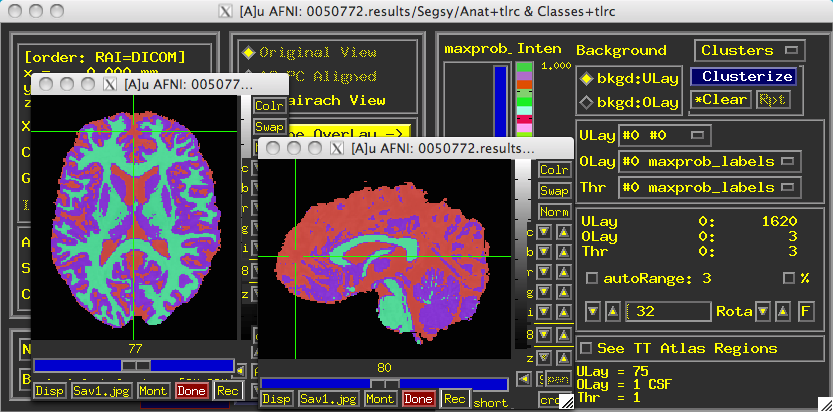
Once it completes, a directory called "Segsy" is generated containing a dataset labeled "Classes+tlrc". Overlaying this over the anatomical looks something like this:
Note that each tissue class assigned both a string label and a number. The defaults are:
1 = CSF
2 = Grey Matter
3 = White Matter
To extract any one of these individually, you can use the "equals" operator in 3dcalc:
3dcalc -a Classes+tlrc -expr 'equals(a, 3)' -prefix WM
This would extract only those voxels containing a 3, and dump them into a new dataset, which I have here called WM, and assign those voxels a value of 1; much like making any kind of mask with FMRI data.
Once you have your tissue mask, you need to first resample it to match the grid for whatever dataset you are extracting data from:
3dresample -master errts.0050772+tlrc -inset WM+tlrc -prefix WM_Resampled
You can then extract the average signal at each timepoint in that mask using 3dmaskave:
3dmaskave -quiet -mask WM_Resampled+tlrc errts.0050772 > WM_Timecourse.1D
This resulting nuisance regressor, WM_Timecourse.1D, can then be thrust into your model with the -stim_files option in 3dDeconvolve, which will not convolve it with any basis function.
To check whether the average timecourse looks reasonable, you can feed the output from the 3dmaskave command to 1dplot via the-stdin option:
3dmaskave -quiet -mask WM_Resampled+tlrc errts.0050772 | 1dplot -stdin
All of this, along with a new shirt I purchased at Express Men, is shown in the following video.
*There are a few, such as Yarkoni et al, 2009, who have found results suggesting that BOLD responses can be found within white matter, but for the purposes of this post I will assume that we all think the same and that we all believe that BOLD responses can only occur in grey matter. There, all better.