DTI Analysis: Soup to Nuts Playlist

Instead of going through each DTI analysis step individually, I've collated everything into a Youtube playlist down below. Just remember that we are using data from the FSL practical course here, and also remember that suing somebody for giving out bad advice, although it is admittedly an easy way to become fantastically wealthy, won't necessarily make you happier.

In any case, just to briefly go over the rest of the steps: After correcting for magnetic field distortions and eddy currents, tensors are fitted using the dtifit command (or simply going through the FDT menu in the FSL interface). Once this has been done for each subject, a series of TBSS tools are used, each one prefixed by "tbss"; for example, tbss_1_preproc, tbss_2_reg, and so on. (You can find all of these in the $FSLDIR/bin directory, and if you have a good handle on Unix programming, you can inspect the code yourself.) After you have run all of those for your dataset, you set up the appropriate experimental design and contrasts, and use the randomise tool to perform statistics in your tractography mask.

Keep in mind that this is just beginner's material; and that if you were to compare your DTI competence to dating, if would be like you were still in that awkward teenager phase, unable to talk to anybody or make eye contact.

However, much of this material has already been covered in other blogs and online resources, provided by several other highly talented scientists and researchers, and - as much as I constantly fantasize about establishing a monopoly over neuroimaging information - there is no practical way to destroy them all.

Therefore, instead of posting redundant information, I highly recommend checking out an ongoing step-by-step series on TORTOISE by Peter Molfese, which you can compare to your results with FSL, and another blog dedicated to diffusion imaging, diffusion-imaging.com. The latter site covers virtually every piece of diffusion imaging software and pipeline out there, and is a good place to start.

DTI Analysis, Steps 1 & 2: Distortion Correction and Eddy Correction

DTI data comes into this world just as we do - raw, unprocessed, unthresholded, and disgusting. Today's parents are much too easy on their children; back in my day, boys and girls were expected to correct their own erratic motion artifacts, to strip their own skulls when too much cranium started sprouting around their cortex, and reach significance through their own diligence and hard work. "No dinner for you until you've gotten rid of those filthy distortion currents on your hands, young man!" was a common saying around my household.

Unfortunately, these days we live in a society increasingly avoiding taking responsibility for their own actions, filled with people more and more unwilling to strip their own skulls. (Even though that would save neuroimaging researchers countless hours of preprocessing.) This trend is the result of several complex cultural and sociological factors, by which I mean: Lawyers. Things have gotten so bad that you could, to take a random example, potentially sue someone posting advice on an unlicensed website if following those instructions somehow messed up your data.

This actually happened to a friend of mine who publishes the nutrition blog tailored for Caucasian males, White Man's Secret. After one of his readers formed kidney stones as a result of following advice to drink a two-liter of Mello Yello every day, the author was sued for - and I quote from the court petition - "Twelve Bazillion Dollars."

In any case, DTI data takes some time to clean up before you can do any statistics on it. However, the preprocessing steps are relatively few, and are analogous to what is done in a typical FMRI preprocessing pipeline. The steps are to identify and correct any distortions during the acquisition, and then to correct for eddy currents.

The first step, distortion correction, can be done with FSL's topup command. Note that this will require two diffusion weighted images, one with the encoding direction in anterior-to-posterior direction (AP) and one encoded in the posterior-to-anterior direction (PA). You will also need a textfile containing information about the encoding directions and the total readout time (roughly the amount of time between the first echo and the last echo); for example, let's say we have a text file, acqparams.txt, containing the following rows:

0 -1 0 0.0665
0 1 0 0.0665

Here a -1 means AP, and 1 means PA. The last column is the readout time. If you have any questions about this, ask your scanner technician. "What if he's kind of creepy?" I don't care, girl; you gotta find out somehow.

While you're at it, also ask which image from the scan was the AP scan, and which was the PA scan. Once you have identified each, you should combine the two using fslmerge:

fslmerge -t AP_PA_scan AP_scan PA_scan 

Once you have that, you have all you need for topup:

topup --imain=AP_PA_scan --datain=acqparams.txt --out=topup_AP_PA_scan

This will produce an image, topup_AP_PA_scan, of where the distortions are located in your DTI scan. This will then be called by the eddy tool to undo any distortions at the same time that it does eddy correction.

The only other preparation you need for the eddy correction is an index list of where the acquisition parameters hold (which should usually just be a 1 for each row for each scan), and a mask excluding any non-brain content, which you can do with bet:

bet dwi_image betted_dwi_image -m -f 0.2

Then feed this into the eddy command (note that a bvecs and bvals image should be automatically generated if you imported your data using a tool such as dcm2niigui):

eddy --imain=dwi_image --mask=betted_dwi_image --index=index.txt --acqp=acqparams.txt --bvecs=bvecs --bvals=bvals --fwhm=0 --topup=topup_AP_PA_scan --flm=quadratic --out=eddy_unwarped_images

Note that the --fwhm and --flm arguments I chose here are the defaults that FSL recommends.

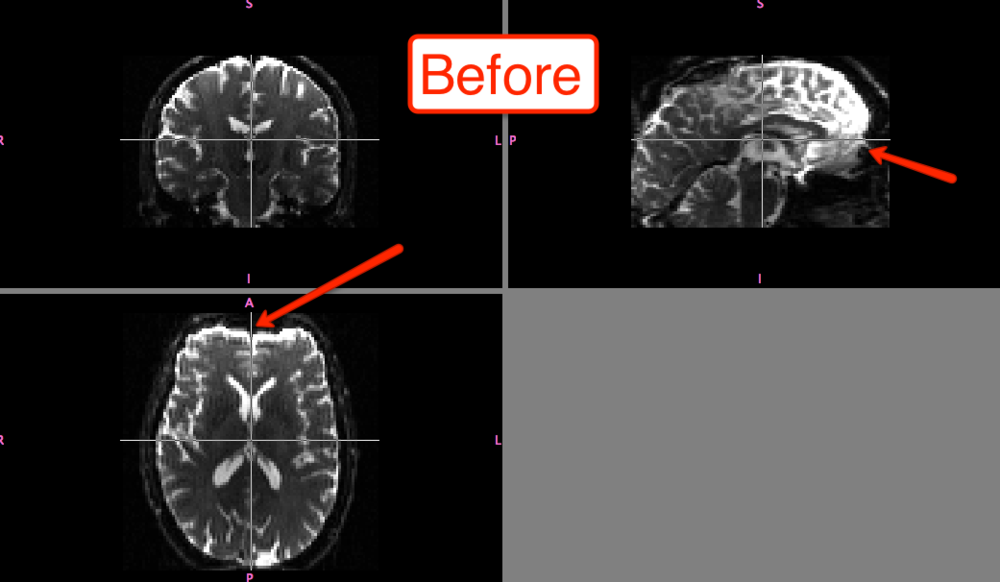
The differences before and after can be seen in fslview:

Of course, the distortion correction step isn't strictly necessary; and you can still do a much simpler version of eddy correction by simply selecting FDT Diffusion from the FSL menu and then selecting the Eddy Correction tab, which only requires input and output arguments. All I'm saying is that, if you're feeling particularly litigious, you should probably be safe and do both steps.

Introduction to Diffusion Tensor Imaging: From Hospital Horror Story to Neuroimaging

It is well known that one of the deepest human fears is to be a patient in a hospital late at night, all alone, while a psychotic nurse injects you with a paralyzing agent, opens up your skull with a bone saw, and begins peeling away layers of your cortex while you are still awake.*

As horrifying as this nightmare scenario may be, it also lends an important insight into an increasingly popular neuroimaging method, diffusion tensor imaging (DTI; pronounced "diddy"). To be more gruesomely specific, the psychotic nurse is able to peel away strips of your brain because it has preferred tear directions - just like string cheese. These strips follow the general direction of fascicles, or bundles of nerves, comprising grey and white matter pathways; and of these pathways, it is white matter that tends to exhibit a curious phenomenon called anisotropy.

Imagine, for example, that I release a gas - such as, let's say, deadly neurotoxin - into a spherical compartment, such as a balloon. The gas, through a process called Brownian motion (not to be confused with the Dr. Will Brown frequently mentioned here) will begin to diffuse randomly in all directions; in other words, as though it is unconstrained.

However, release the same gas into a cylindrical or tube-shaped compartment, such as one of those cardboard tubes you used to fight with when you were a kid,** and the gas particles will tend to move along the direction of the tube. This is what is known as anisotropy, meaning that the direction of the diffusion tends to go in a particular direction, as opposed to isotropy, where diffusion occurs in all directions with equal probability.

Left two figures: Ellipsoids showing different amounts of anisotropy, with lambda 1, 2, and 3 symbolizing eigenvalues. Eigenvalues represent the amount of diffusion along a particular direction. Right: A sphere representing isotropy, where diffusion occurs with equal probability in all directions.

This diffusion can be measured in DTI scans, which in turn can be used to indirectly measure white matter integrity and structural connectivity between different areas of the brain. A common use of DTI is to compare different populations, such as young and old, and to observe where fractional anisotropy (FA) differs between groups, possibly with the assumption that less FA can be indicative of less efficient communication between cortical regions. There are other applications as well, but this is the one we will focus on for the remainder of the tutorials.

The data that we will be using can be found on the FSL course website, after scrolling down to Data Files and downloading File 2 (melodic and diffusion). I haven't been able to find any good online repositories for DTI data, so we'll be working with a relatively small sample of three subjects in one group, and three subjects in the other. Also note that while we will focus on FSL, there are many other tools that process DTI data, including some new commands in AFNI, and also a program called TORTOISE. As with most things I post about, these methods have already been covered in detail by others; and in particular I recommend a blog called blog.cogneurostats.com, which covers both the AFNI and TORTOISE approaches to DTI, along with other tutorials that I thought I had been the first to cover, but which have actually already been discussed in detail. I encourage you to check it out - but also to come back, eventually.

*Or maybe that's just me.
**And maybe you still do!

Introduction to Independent Components Analysis

In the course of your FMRI studies, you may have at one point stumbled upon the nightmarish world of Independent Components Analysis (ICA), an intimidating-sounding technique often used by people who know far more than I do. Nevertheless, let us meditate upon it and see what manner of things we have here.

Components are simpler building blocks of a more complex signal. For example, in music, the soundwave profiles of chords can appear very complex; yet a Fourier analysis can filter it back into its constituent parts - simpler sine waves associated with each note that, combined together, create the chord's waveform.

A similar process happens when ICA is applied to neuroimaging data. Data which comes right off the scanner is horribly messy, a festering welter of voxels and timecourses that any right man would run away from as though his very life depended upon it. To make this more comprehensible, however, ICA can decompose it into more meaningful components, each one explaining some amount of the variance of the overall signal. 

Note also that we talk of spatial and temporal components, which will be extracted from each other; this may seem somewhat odd, as the two are inseparable in a typical FMRI dataset: each voxel (the spatial component) has a timecourse (the temporal component). However, ICA splits these apart and recombines them, in descending order, into components that explain the amount of variance of the original spatio-temporal maps. This is what is represented in the figures shown on the FSL website, reprinted below:

After these components have been extracted, something happens that some (like me) consider terrifying: You need to identify the components yourself, assigning each one to whatever condition seems most reasonable. Does that one look like a component related to visual processing? Then call it the visual component. Does that one look like a resting-state network? Then call it a resting-state network component. This may all seem rather cavalier, especially considering that you are the one making the judgments. Seriously; just think about that for a moment. Think about what you've done today.

In any case, that is a brief overview of ICA. To be fair, there are more rigorous ways of classifying what components actually represent - such as creating templates for connectivity networks or activation patterns and calculating the amount of fit between that and your component - but to be honest, you probably don't have the motivation to go through all of that. And by you, I mean me.

Next we will work through the example datasets on FSL's website, discussing such problems as over- and under-fitting, the Melodic GUI, and what options need to be changed; followed by using ICA to analyze resting-state data.

Automating 3dReHo

As a rider to our tale of Regional Homogeneity analysis, we last discuss here how to automate it over all the subjects of your neuroimaging fiefdom. Much of this will look similar to what we have done with other analyses, but in case you don't know where to start, this should help get you going.


#!/bin/tcsh

setenv mask mask_group #Set your own mask here
setenv subjects "0050773 0050774" #Replace with your own subject numbers within quotations

foreach subj ($subjects)

cd {$subj}/session_1/{$subj}.results #Note that this path may be different for you; change accordingly

3dReHo -prefix ReHo_{$subj} -inset errts.{$subj}+tlrc -mask mask_group+tlrc #Perform Regional Homogeneity analysis

#Convert data to NIFTI format
3dAFNItoNIFTI ReHo_{$subj}+tlrc.HEAD
3dAFNItoNIFTI {$mask}+tlrc.HEAD

#Normalize images using FSL commands
setenv meanReHo `fslstats ReHo_{$subj}.nii -M`
setenv stdReHo `fslstats ReHo_{$subj}.nii -S`

fslmaths ReHo_{$subj}.nii -sub $meanReHo -div $stdReHo -mul mask_group.nii ReHo_Norm_{$subj}

gunzip *.gz

#Convert back to AFNI format
3dcopy ReHo_Norm_{$subj}.nii ReHo_Norm_{$subj}

end

ReHo Normalization with FSL

As a brief addendum to the previous post, ReHo maps can also be normalized using FSL tools instead of 3dcalc. Conceptually, it is identical to what was discussed previously; however, the ability to set variables as the output of FSL commands makes it more flexible for shell scripting. For example, using the same datasets as before, we could set the mean and standard deviation to variables using the following combination of AFNI and FSL commands:

3dAFNItoNIFTI ReHo_Test_Mask+tlrc
3dAFNItoNIFTI mask_group+tlrc

setenv meanReHo `fslstats ReHo_Test_Mask.nii -M`
setenv stdReHo `fslstats ReHo_Test_Mask.nii -S`
fslmaths ReHo_Test_Mask.nii -sub $meanReHo -div $stdReHo -mul mask_group.nii ReHo_Norm
gunzip *.gz
3dcopy ReHo_Norm.nii ReHo_Norm


An explanation of these commands is outlined in the video below. Also, suits!

Future Functional Connectivity Tutorials, and Other Updates

A few notes:

1) The previous functional connectivity posts and tutorials are cribbed from Gang Chen's homepage, which is available here. Kind of like the way I crib quotations and passages from authors that no one reads anymore, and then pass it off as my own style to boost my pathologically low self-esteem. Keep in mind that most of these demonstrations deal with a single subject and simplified situations that you probably will not encounter in your research. Given these contrived examples, most of the results generated in these demos are relatively meaningless; it's up to you to learn and understand the concepts, and then apply them to your own data and make your own inferences. My task which I am trying to achieve is, by the power of Youtube tutorials, to make you hear, to make you feel — it is, before all, to make you understand. That — and no more, and it is everything. (That was Conrad, by the way.)

2) A lot of you - I'm talking a LOT of you players - have been making requests for MELODIC tutorials and resting state analyses in FSL. All I can say is, we'll get there, in time. Before that, however, I believe AFNI is better suited for building up one's intuition, and so we will be working through a few more connectivity topics in AFNI - specifically, context-dependent correlations, beta series correlations, and resting state connectivity. After that we will again cover the same concepts, but applied in FSL - by which time, given my glacial pace, either FMRI will have become a passé technique or the Andromeda galaxy will have crashed into us.

3) Recently you may have noticed the "Donate" button on the right sidebar of the blog. This was done at the request of one reader who felt the powerful, irrational urge to loosen his purse-strings and give some alms out of the goodness of his heart, which is located somewhere way, way down there, somewhere nearabouts the cockles. Although I can't fully understand this behavior - even less than I can understand why there is someone who still has purse-strings, or what cockles are, exactly - nevertheless it helps satisfy my cupidity and strokes my ego. Furthermore, in addition to serving Mammon, these tokens of gratitude motivate me to regularly produce new material and, as a bonus, help me to continue procrastinating on my dissertation. Now that's what I call a win-win-win.

4) Also, at least one of you has mailed me a two-pack of Nutella. This has pleased me greatly. My brain needs hazelnut spread for fuel, and the more it has, the hotter and better it burns.

5) If everything goes according to plan, we should cover context-dependent correlations this weekend, beta series correlations next week, and resting-state connectivity the week after that.

Lunch in Paris, dinner in London, comrade.

Combining ROIs

Once you've used a tool like fslmaths, 3dcalc, or Marsbar to create a single ROI, you can combine several of these ROIs using the same tools. This might be useful, for example, when creating a larger-scale masks encompassing several different areas.

In each case, combining ROIs is simply a matter of creating new images using a calculator-like tool; think of your TI-83 from the good old days, minus those frustrating yet addictive games such as FallDown. (Personal record: 1083.) With fslmaths, use the -add flag to concatenate several different ROIs together, e.g.:

fslmaths roi1 -add roi2 -add roi3 outputfile

With AFNI:

3dcalc -a roi1 -b roi2 -c roi3 -expr '(a+b+c)' -prefix outputfile

With Marsbar is a bit more involved, but also easier since you can do it from the GUI, as shown in the following video.




Many thanks to alert reader Anonymous, who is both too cool to register a username and once scored a 1362 on FallDown. Now all you gotta do is lay back and wait for the babe stampede!

Parameter Extraction in AFNI: 3dmaskave and 3dmaskdump

Previously we showed how to extract parameters using Marsbar in SPM and featquery in FSL, and the concept is identical for AFNI. Once you have created a mask (e.g., using 3dUndump or 3dcalc), you can then extract parameter estimates from that ROI either using the tool 3dmaskave or 3dmaskdump.
3dmaskave is quicker and more efficient, and is probably what you will need most of the time. Simply supply a mask and the dataset you wish to extract from, and it will generate a single number of the average parameter estimate across all the voxels within that ROI. For example, let's say that I want to extract beta weights from an ROI centered on the left nucleus accumbens, and I have already created a 5mm sphere around that structure stored in a dataset called LeftNaccMask+tlrc. Furthermore, let's say that the beta weights I want to extract are in a beta map contained in the second sub-brik of my statistical output dataset. (Remember that in AFNI, sub-briks start at 0, so the "second" sub-brik would be sub-brik #1.) To do this, use a command like the following:

3dmaskave -mask LeftNaccMask+tlrc stats.202+tlrc'[1]'

This will generate a single number, which is the average beta value across all the voxels in your ROI.

The second approach is to use 3dmaskdump, which provides more information than 3dmaskave. This command will generate a text file that contains a single beta value at each voxel within the ROI. A couple of useful options are -noijk, to suppress the output of voxel coordinates in native space, and -xyz, to output voxel coordinates in the orientation of the master dataset (usually in RAI orientation). For example, to output a list of beta values into a text file called LeftNaccDumpMask.txt,

3dmaskdump -o LeftNaccDumpMask.txt -noijk -xyz -mask LeftNaccMask+tlrc stats.202+tlrc'[1]'

This will produce a text file that contains four columns: The first three columns are the x-, y-, and z-coordinates, and the fourth column is the beta value at that triplet of coordinates. You can take the average of this column by exporting the text file to a spreadsheet like Excel, or use a command like awk from the command line, e.g.

awk '{sum += $4} END {print "Average = ", sum/NR}' LeftNaccDumpMask.txt


Keep in mind that this is only for a single subject; when you perform a second-level analysis, usually what you will want to do is loop this over all of the subjects in your experiment, and perform a statistical test (e.g., t-test) on the resulting beta values.






Concluding Unscientific Postscript

I recently came across this recording of Schubert's Wanderer Fantasie, and I can't help but share it here; this guy's execution is damn near flawless, and, given both the time of the recording and some of the inevitable mistakes that come up, I have good reason to believe it was done in a single take. It's no secret that I do not listen to that much modern music, but it isn't that modern music is bad, necessarily; it's just that classical music is so good. Check out the melodic line around 16:30 to hear what I'm talking about.

FSL Tutorial: Creating ROIs from Coordinates

Previously we covered how to create regions of interest (ROIs) using both functional contrasts and anatomical landmarks; however, FSL can also create spheres around voxel coordinates, similar to AFNI's 3dcalc or SPM's marsbar.

1. Step one is to find the corresponding voxel coordinates for your MNI coordinates, which may be based on peak voxel activation from another study, for example; to do this, open up FSLview, type in your MNI coordinates, and write down the corresponding voxel coordinates (these are shown in the bottom-left corner of FSLview). 
2. After you have written down your voxel coordinates, create a point at those coordinates using the fslmaths command. This command requires the template space that you warped to, as well as the actual x-, y-, and z-coordinates corresponding to the MNI coordinates. Give the output file a name, and make sure that the output data type ('odt') is set to float. (Example command: fslmaths avg152T1.nii.gz -mul 0 -add 1 -roi 45 1 74 1 51 1 0 1 ACCpoint -odt float)
3. Using fslmaths again, input the file containing the point created in the previous step, and specify a sphere of radius N (in millimeters) to expand around that point. Use the -fmean command, for reasons that are to remain mysterious, and provide a label for your output data set. (Example command: fslmaths ACCpoint -kernel sphere 5 -fmean ACCsphere -odt float)
4. Update on 5/18/2016: To make it a binary mask, execute one more command: fslmaths ACCsphere.nii.gz -bin ACCsphere_bin.nii.gz. The previous step creates a sphere, but with small intensities; this can be problematic if you do a featquery analysis that allows weighting of the image.

Once that is all done, use fslview to open up a template in your normalized space, and overlay your newly created sphere; double-check to make sure that it is in roughly the location where you think it should be. Now you can extract data such as parameter estimates from this ROI, using techniques similar to those covered in previous tutorials about ROIs.

Thanks to alert viewer danieldickstein, which, due to its juvenile reference to the male member, cannot possibly be his real name. Grow up, Daniel.