FSL Summary

After finishing that cycle of tutorials, I feel as though a summary would be useful. Some of these are points that were highlighted during the walkthroughs, whereas others are germane to any neuroimaging experiment and not necessarily specific to any software analysis package. The past couple of weeks have only scratched the surface as to the many different experimental approaches and analysis techniques that are available, and the number of ways to gather and interpret a set of data are nearly inexhaustible.

That being said, here are some of the main points of FSL:

1) These guys really, really like acronyms. If this pisses you off, if you find it more distracting than useful, I'm sorry.

2) Download a conversion package such as dcm2nii (part of Chris Rorden's mricron package here) in order to convert your data into nifti format. Experiment with the different suffix options in order to generate images that are interpretable and easy to read.

3) Use BET to skull strip your anatomicals as your first step. There is an option for using BET within the FEAT interface; however, this is for your functional images, not your anatomical scans. Skull stripping is necessary for more accurate coregistration and normalization, or warping your images to a standardized space.

4) As opposed to other analysis packages, FSL considers each individual run to be a first-level analysis; an individual subject comprising several runs to be a second-level analysis; collapsing across subjects to be a third-level analysis; and so forth. I recommend using the FEAT interface to produce a template for how you will analyze each run (and, later, each subject), before proceeding to batch your analyses. Especially for the beginner, using a graphical interface is instructive and helps you to comprehend how each step relates to the next step in the processing stream; however, once you feel as though you understand enough about the interface, wean yourself off it immediately and proceed to scripting your analyses.

5) Use the Custom 3-column option within the Stats tab of FEAT in order to set up your analysis. Most studies these days are event-related, meaning that events are of relatively short duration, and that the order of presentation is (usually) randomized. Even if your analysis follows the same pattern for each run, it is still a good habit to use and get comfortable with entering in 3-column timing files for your analysis.

6) If your initial attempts at registration and normalization fail, set the coregistration and normalization parameters to full search and maximum degrees of freedom (i.e., 12 DOF). This takes more time, but has fixed every registration problem I have had with FSL.

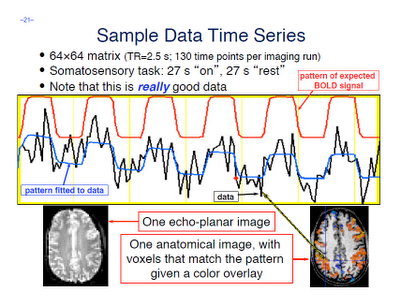
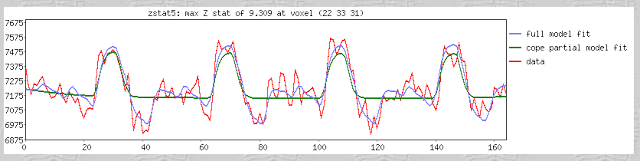
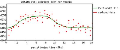
7) Look at the output from your stats, and make sure they are reasonable. If you have done a robust contrast which should produce reliable activations - such as left button presses minus right button presses - make sure that it is there. If not, this suggests a problem with your timing, or with your images, which is a good thing to catch early. Also look at your design matrix, and make sure that events are lined up when you think they should be lined up; any odd-looking convolutions should be investigated and taken care of.

8) This piece of advice was not covered in the tutorials, nor does it apply to neuroimaging analysis itself exactly, but it bears repeating: Run a behavioral experiment before you scan. Obtaining behavioral effects - such as reaction time differences - are good indicators that there may actually be something going on neurally that is causing the observed effects. The strength and direction of these behavioral differences will allow you to predict and refine your hypotheses about where you might observe activation, and why. Furthermore, behavioral experiments are much cheaper to do than neuroimaging experiments, and can lead to you to make considerable revisions to your experimental paradigm. Running yourself through the experiment will allow you to make a series of commonsense but important judgments, such as: Do I understand how to do this task? Is it too long or too boring, or not long enough? Do I have any subjective feeling about what I think this experiment should elicit? It may drive you insane to pilot your study on yourself each time you make a revision, but good practice, and can save you much time and hassle later.


That's about it. Again, this is targeted mainly toward beginners and students who have only recently entered the field. All I can advise is that you stick with it, take note of how the top scientists run their experiments, and learn how to script your analyses as soon as possible. It can be a pain in the ass to learn, especially if you are new to programming languages, but it will ultimately save you a lot of time. Good luck.

FSL Tutorial 6: Automating FEAT

So now you know enough to run an analysis on your own; Congratulations! However, before you crack open a fresh jar of Nutella to celebrate, be aware that there are other methods that can greatly increase your efficiency, confidence, and libido.

We now turn to a slightly more sophisticated way to run your analyses, that is, through the command line as opposed to the pointing and clicking through the graphical user interface. When I mentioned in the last post that this factors out human error, what I meant was that it eliminates any error due to faulty clicks in the GUI, or fat-finger dialing of any additional parameters. The probability that you would enter everything in by hand the exact same way for every subject is essentially zero. Learning the basics of scripting is essential for any neuroimaging researcher these days, even if it is just to acquire enough familiarity to know what is going on when reading other people's scripts.

Whenever you set up and run an analysis, a file called design.fsf is output into each results directory; this contains everything you specified in the GUI, but in text format. This file can also be generated at any time by using the "Save" option within the FEAT GUI, and conversely, can be loaded using the "Load" option; this will fill in all of the fields as they were when you saved the design.fsf file.

The power of design.fsf comes from its commandline use. Simply type in "feat design.fsf" and it will execute every command inside the design.fsf file, the same as it would if you were to load it into the FEAT GUI and press the Go button.

Honestly, I am surprised that this feature is not showcased more in the FSL documentation; a couple of lines are devoted to its commandline usage in the FEAT basics section of the manual, but really they should emphasize this much more. (There is a good tutorial here about how to swap code within the design.fsf file and execute it with feat.) If you are new to Unix and need to get your feet wet, I suggest going through the following tutorials: One for basic Unix usage, the other for basics of shells scripting. This will be a new language to you, and as with any language, the beginning can be disorienting and overwhelming at times; however, stick with it, and I promise that the fog will begin to clear eventually, and you will discern what exactly it is you need to know when searching the help manuals, and what it is that you can disregard.

For those of you who have enough Unix background to feel comfortable reading scripts, here is something I created for a recent study I analyzed. This is a special case, since there were some runs where the participant was not exposed to a condition; in this case, for that regressor FSL requires you to specify the shape as "All Zeroes", something that we did not cover yet, but something that you should be aware of. The following script will check for whether the timing file is empty or not, and adjust the shape specification accordingly; however, it will also work for studies which have all regressors accounted for and do not have any missing data.

Here is the script, which can also be downloaded here; I apologize that the formatting is a little screwy with the margins:

#!/bin/bash

for run in 01 02 03 04

do

#Loops through all runs and replaces "ChangeMe" with run number

\cp design.fsf tmpDesign.fsf

sed -i -e 's/run01/runChangeMyRun/' tmpDesign.fsf

sed -i -e 's/FSL_01/FSL_ChangeMyRun/' tmpDesign.fsf #Replaces run placeholder with variable "ChangeMyRun"; this will be swapped later with the appropriate run number

iter=1 #Counter for running loops below

while [ $iter -le 11 ]

do

for timingFile in FSL_"$run"_EmotionRegAM.txt FSL_"$run"_EmotionRegAS.txt FSL_"$run"_EmotionRegNM.txt FSL_"$run"_EmotionRegNS.txt FSL_"$run"_EmotionResp1.txt FSL_"$run"_EmotionResp2.txt FSL_"$run"_EmotionResp3.txt FSL_"$run"_EmotionResp4.txt FSL_"$run"_EmotionResp5.txt FSL_"$run"_Instructions.txt FSL_"$run"_Relax.txt

do

if [ -s ../Timing/$timingFile ]

then

echo "File found; timing file is " $timingFile

sed -i -e 's/fmri(shape'$iter') 3/fmri(shape'$iter') 3/' tmpDesign.fsf

else

echo "File not found; timing file is " $timingFile

sed -i -e 's/fmri(shape'$iter') 3/fmri(shape'$iter') 10/' tmpDesign.fsf

fi

iter=$(( $iter + 1))

done

done

\cp tmpDesign.fsf design_$run.fsf #Make a copy for each run

sed -i -e 's/ChangeMyRun/'$run'/' design_$run.fsf #Swap "ChangeMyRun" with run number

\rm *-e #Remove excess schmutz

feat design_$run.fsf #Run feat for each run

done

Note that a template script is generated by copying a script output by FEAT and replacing "run01" with "runChangeMyRun". ChangeMyRun serves as a placeholder for the run number, being updated on each successive iteration of the loop. The script then executes a while loop, checking each timing file for emptiness, and if it is empty, assigning the appropriate shape in the model. Also note that my timing files, in this example, are located in a directory one level above called "Timing"; this may be different for you, so adjust accordingly if you plan on adapting this script for your purposes.

After that, a new design.fsf is generated for each run, and then executed with feat. If you have more than one subject, then it is a matter of adding another loop on top of this one and going through subjects; with higher-level analyses, replacing single runs of data with .gfeat directories; and so on.

For the beginner, I would recommend opening up a generic design.fsf file with a text editor and using search and replace to update it to the next run. After you get a feel for what is going on, spend some time with Unix and monkey around with the "sed" search and replace tool, until you feel comfortable enough to use it on your design.fsf files; then experiment with loops, and test it on a single subject in a copy directory, so that if something blows up (which it inevitably will on your first go-around), you have a backup.

That is it for the basics of FEAT, and, really, all you need to know for carrying out basic analyses in FSL. Interpreting the results is another matter entirely, but once you have the techniques down, a major part of the drudge work is out of the way, and you can spend more time thinking about and looking at your data; which, really, is what we are trained to do in the first place.

More tutorials will be up soon about the basics of Unix, with an eye on assisting the beginning neuroimaging researcher understand what the hell is going on.

FSL Tutorials 4-5: Group-Level Analysis

It has well been said that analyzing an fMRI dataset is like using a roll of toilet paper; the closer you get to the end, the faster it goes. Now that you know how to analyze a single run, applying this concept to the rest of the dataset is straightforward; simply apply the same steps to each run, and then use the "Higher-Level Analysis" option within FEAT to select your output directories. You might want to label them for ease of reference, with the run number appended to each directory (e.g., output_run01, output_run02, etc).

Also uploaded is a walkthrough for how to locate and look at your results. The main directory of interest is the stats folder, which contains z-maps for each contrast; simply open up fslview and underlay an anatomical image (or a standard template, such as the MNI 152 brain, if it is a higher-level analysis that has been normalized), and then overlay a z-map to visualize your results. The sliders at the top of fslview allow you to set the threshold for the lower and upper bounds of your z-scores, so that, for example, you only see z-scores with a value of 3.0 or greater.

After that, the same logic applies to collapsing parameter estimates across subjects, except that in this case, instead of feeding in single-run FEAT directories into your analysis, you use the GFEAT directories output from collapsing across runs for a single subject. With the use of shell scripting to automate your FEAT analyses, as we will discuss in the next tutorial, you can carry out any analysis quickly and uniformly; not only is scripting an excellent way to reduce the amount of drudge work, but it also ensures that human error is out of the equation once you hit the go button.

Make sure to stay tuned for how to use this amazing feature, therewith achieving the coveted title of Nerd Baller and Creator of the Universe.

FSL Tutorial 3: Running The Analysis

The end of our last set of tutorials covered the FEAT interface; and although there is much more there to explore and use, such as MELODIC's independent component analysis, for now we will simplify things and focus on a traditional, straightforward univariate analysis.

A few terms are worth defining here. First, whenever you read an instruction manual outlining how to set up and run a model with fMRI data, you will inevitably run into the term voxel-wise analysis. (Maybe not inevitably, but the point is, enough researchers and software packages use it to merit an acquaintance with it.) What this means is that we first construct a model of what we believe will happen at each voxel in the brain, given our timing files of what happened when. If, for example, ten seconds into the experiment the subject pressed a button with his right hand, we would expect to see a corresponding activation in the left motor cortex. When we talk about activation, we simply mean whether our model is a good fit or not for the signal observed in that voxel; and this model is generated by convolving - also known as the application of a moving average, a concept which is more easily explained through an animation found here - each event with a basis function, the most common and intuitive of which is a gamma function. Essentially what this boils down to is pattern matching in time; the better the fit for a particular contrast or condition, the more likely we are to believe that that particular voxel is responsive to that condition.

This image was stolen (literally) from the AFNI website educational material. Note that the red line is the ideal fit, while the blue line is the ideal fit scaled by a certain amount in order to fit the data. These scalars are also called beta weights; we will have "The Talk" about these at a later time, but only after you have reached fMRI maturity.

Furthermore, within the output of FEAT you will see plotted timecourses for each peak voxel for each contrast. The red line represents the raw signal timeseries at that voxel, which, as you can see, is relatively noisy, although it is clear when certain conditions were present. It should be noted that this experiment is a special case, as we are dealing with a block design which elicits robust activation in the left and right motor cortices; most studies employing event-related designs have much noisier data which is much more difficult to interpret. The blue line represents the complete model fit; that is, given all of the regressors, whether any activation in this voxel can be attributed to any of your conditions. Lastly, the green line represents only the contrast or condition of interest, and is usually only meaningful when looking at simple effects (i.e., undifferentiated contrasts which compare only one condition to the baseline signal present in the data).

One feature not covered in this video tutorial is the visualization of peristimulus plots, which allow the user to see averages of the event over multiple repetitions. It provides much of the same information as the basic timeseries plots, but from a slightly different vantage point; you can see what timepoints are averaged, exactly, and how this contributes to the observed model fit.

Now that you have had FEAT guide you by the hand through your results, it is time to get down and dirty and look at your results in the output directories by yourself. FEAT generates a lot of output, but only a fraction of it is worth investigating for the beginning researcher, and almost all of it can be found in the stats directory. We will cover this in the following tutorial; for now, check your freezer for Hot Pockets.

FSL Tutorial 2: FEAT (Part 3): For The Wind

Pictured: FSL User

[Before we begin: According to my traffic sources, the majority of my viewers, outside of the United States, are from Russia. If the history books I have read and the video games I have played are any guide, they are probably visiting this site in order to learn enough about cognitive neuroscience to produce some kind of supersoldier in order to restore communist hardliners to power and launch an assault on America. So, to all of my Russian readers: Hola!]

Finally, we have arrived at the end of the FEAT interface. The last two tabs, post-stats and registration, allow the user to specify how the results will be visualized, what kinds of multiple comparison corrections to carry out, and how to register and normalize the data.

One might wonder why FSL chooses to perform coregistration and normalization as the last step, instead of at a previous step in the preprocessing pipeline as do other software analysis packages. The reasoning is that because these steps introduce spatial correlations, it is better to introduce them after having run the statistical analysis, in order to prevent any sort of biases that may be introduced into the data as a result of applying these steps. Personally, I don't think it matters that much either way, since you have to do it at some point; however, that is the way it is built into the FSL stream, and if you don't like it, tough bananas.

Most of the defaults are fine; the only tab that requires any input before you can move forward is the Registration tab, which requires a skullstripped brain to normalize to a standardized space. This includes atlases such as Talairach or Montreal Neurological Institute (MNI), although I believe FSL only uses MNI. The point of normalization is that every subject's brain will be twisted, rotated, warped, and undergo various other uncomfortable transformations until it is located within a box that has equal dimensions to the standard space. Furthermore, certain anatomical landmarks will be at a specific coordinate position relative to every other part of the brain; for example, in Talairach space, the anterior commissure - a bundle of nerve fibers connecting the hemispheres, located at the base of the anterior columns of the fornix - will be positioned at coordinates 0, 0, 0. Thus, according to the Talairach atlas in this example, any other brain regions can be defined based on their distance from this origin (although the researcher should always check to make sure that what the atlas says matches up with what is directly in front of him).

A couple of other useful options are in the post-stats tab. For example, Pre-threshold masking allows the user to perform region of interest (ROI) analyses which define an a priori region either based on anatomical regions defined by an atlas or a binary mask generated by a program like Marsbar. Contrast masking has a similar role, masking out certain regions of the brain based on whether they are covered by another contrast in the analysis; although caution should be exercised here as well, in order to make sure that the masking contrast is orthogonal to the one being investigated. For more information about ROI analyses, as well as potential pitfalls, see an earlier post about the topic.

More tutorials will be up soon to guide the user through what all those HTML output files mean, as well as looking at and interpreting results.

FSL Tutorial 2: FEAT (Part 2): The Reckoning

(Note: Hit the fullscreen option and play at a higher resolution for better viewing)

Now things get serious. I am talking more serious than the projected peak Nutella in 2020, after which our Nutella resources will slow down to a trickle and then simply evaporate. This video goes into detail about the FEAT stats tab, specifically what you should and shouldn't do (which pretty much means just leaving most of the defaults as is), lest you screw everything up, which, let's face it, you probably will anyway. People will tell you that's okay, but it's not.

I've tried to compress these tutorials into a shorter amount of time, because I usually take one look at the duration of an online video and don't even bother with something greater than three or four minutes (unless it happens to be a Starcraft 2 replay). But there's no getting around the fact that this stuff takes a while to explain, so the walkthroughs will probably remain in the ten-minute range.

To supplement the tutorial, it may help to flesh out a few concepts, particularly if this is your first time doing stuff in FSL. The most important part of an fMRI experiment - besides the fact that it should be well-planned, make sense to the subject, and be designed to compare hypotheses against each other - is the timing. In other words, knowing what happened when. If you don't know that, you're up a creek without Nutella a paddle. There's no way to salvage your experiment if the timing is off or unreliable.

The documentation on FSL's website isn't very good when demonstrating how to make timing files, and I'm surprised that the default option is a square waveform to be convolved with a canonical Hemodynamic Response Function (HRF). What almost every researcher will want is the Custom 3 Column format, which specifies the onset of each condition, how long it lasted, and any auxiliary parametric information you have reason to believe may modulate the amplitude of the Blood Oxygenation Level Dependent (BOLD) response. This auxiliary parametric information could be anything about that particular trial of the condition; for example, if you are showing the subject one of those messed-up IAPS photos, and you have a rating about how messed-up it is, this can be entered into the third column of the timing file. If you have no reason to believe that one trial of a condition should be different from any other in that condition, you can set every instance to 1.

Here is a sample timing file to be read into FSL (which they should post an example of somewhere in their documentation; I haven't been able to find one yet, but they do provide a textual walkthrough of how to do it under the EV's part of the Stats section here):

10  1  1
18  1  1
25  1  1
30  1  1


To translate this text file, this would mean that this condition occurred at 10, 18, 25, and 30 seconds relative to the start of the run; each trial of this condition lasted one second; and there is no parametric modulation.

A couple of other things to keep in mind:

1) When setting up contrasts, also make a simple effect (i.e., just estimate a beta weight) for each condition. This is because if everything is set up as a contrast of one beta weight minus another, you can lose valuable information about what is going on in that contrast.

As an example of why this might be important, look at this graph. Just look at it!

Proof that fMRI data is (mostly) crap

These are timecourses extracted from two different conditions, helpfully labeled "pred2corr0" and "pred2corr1". When we took a contrast of pred2corr0 and compared it to pred2corr1, we got a positive value. However, here's what happened: The peaks of the HRF (represented here by the timepoints under the "3" in the x-axis, which translates into 6 seconds (3 scans of 2 seconds each = 6 seconds), representing the typical peak of the HRF after the onset of a stimulus) for both conditions were negative. It just happened that the peak for the pred2corr1 condition was more negative than that of pred2corr0, hence the positive contrast value.

2) If you have selected "Temporal Derivative" for all of your regressors, then every other column will represent an estimate of what the temporal derivative should look like. Adding a temporal derivative has the advantage of accounting for any potential lags in the onset of the HRF, but comes at the cost of a degree of freedom, since you have something extra to estimate.

3) After the model is set up and you click on the "Efficiency" tab, you will see two sections. The section on the left represents the correlation between regressors, and the section on the right represents the singular value decomposition eigenvalue for each condition.

What is an eigenvalue? Don't ask me; I'm just a mere cognitive neuroscientist.

For the correlations, brighter intensities represent higher correlations. So, it makes sense that the diagonal is all white, since each condition correlates with itself perfectly. However, it is the off-diagonal squares that you need to pay attention to, and if any of them are overly bright, you have a problem. A big one. Bigger than finding someone you loved and trusted just ate your Nu-...but let's not go there.

As for the eigenvalues on the right, I have yet to find out what range of values represent safety and which ones represent danger. I will keep looking, but for now, it is probably a better bet to do design efficiency estimation using a package like AFNI to get a good idea of how your design will hold up under analysis.


That's it. A few more videos will be uploaded, and then the beginning user should have everything he needs to get started.

FSL Tutorial 2: FEAT (Part 1)

A new tutorial about FEAT is now up; depending on how long it takes to get through all of the different tabs in the interface, this may be a three-part series. In any case, this will serve as a basic overview of the preprocessing steps of FEAT, most of which can be left as a default.

The next couple of tutorials will cover the set up of models and timing files within FSL, which can be a little tricky. For those of you who have stuck with it from the beginning (and I have heard that there are a few of you out there: Hello), there will be some more useful features coming up, aside from reviewing the basics.

Eventually we will get around to batch scripting FEAT analyses, which can save you several hours of mindless pointing and clicking, and leave you with plenty of time to watch Starcraft 2 replays, or Breaking Bad, or whatever it is kids watch these days.

FSL Tutorial: Part 1 (of many)

I recently started testing out FSL to see if it has any advantages over other fMRI analysis packages, and decided to document everything on Youtube as I go along. The concepts are the same as any other package (AFNI, SPM, etc), but the terminology is slightly different, and driving it from the command line is not as intuitive as you would think. Plus, they use a ton of acronyms for everything, which, to be honest, kind of pisses me off; I don't like it when they try to be cute and funny like that. The quotes and sonnets generated by AFNI after exiting the program, however, are sophisticated and endearing. One of my favorites: "Each goodbye makes the next hello closer!"

In any case, here is the first, introductory tutorial I made about FSL. I realized from searching around on Youtube that hardly any fMRI analysis tutorial videos exist, and that this is a market that sorely needs to be filled. A series of walkthroughs and online lessons using actual data, in my opinion, would be far more useful at illustrating the fundamentals of fMRI data analysis than only having manuals (although those are extremely important as well, and I would recommend that anyone getting started in the field read them so that they can needlessly suffer as I did).

I will attempt to upload more on a regular basis, and start to get some coherent lesson plan going which allows the beginner to get off the ground and understand what the hell is going on. True story: It took me at least three years to fully comprehend what a beta weight was. Three years. I'm not going to blame it all on Smirnoff Ice, but it certainly didn't help.

Note: I suggest hitting fullscreen mode and viewing at a higher resolution (360p or 480p) in order to better see the text in the terminal window.

Also, the example data for these tutorials can be found here.