SPM Design Specification and Estimation

At long last, after several long minutes - perhaps hours - or grueling preprocessing, you are ready to specify your general linear model. The concept is straightforward enough: Specify when a certain condition happened, input how long that condition took to happen (zero duration in the case of an instantaneous event), and what kind of basis function you want to convolve with that condition. Basis functions is a topic all on its own (you'll find out more when you're older!), but for the time being, realize that the canonical hemodynamic response function will suffice for most of your cases; even though sometimes it is a laughably wrong assumption about the shape of your hemodynamic response. But hey, it's the best we've got.

More details on the ins and outs of model specification, along with an example of what might be going through your head as you do this, can be found in the following video.


SPM Official (!) Videos

Now in video form!


I don't know how I missed this, but apparently there are official SPM videos up on the SPM website (if you can believe it) - very similar to what I have been producing the past few months. It still eludes me how they managed to steal my idea over a year before I implemented it, but there you go. I haven't actually watched the casts; more like, I've skipped around to a few points in each, with the sound off, because I'm considerate and I don't want to disturb my labmates. (They have also threatened to beat me up and give me a swirly if I unmuted the volume on my computer.)

In any case, although conspicuously lacking the raw sex appeal of my tutorials, these guys still seem to do a good job in explaining the software and the concepts behind it, even if they do tend to speak at times with an accent. "If the sound is off, how do you know they speak with an accent?" It's called being cultured. (Turns up Enya; begins getting pummeled by labmates.)


A link to the videos can be found here; not that I'm insecure or anything, but please don't allow them to replace me.

Smoothing in SPM: The Do's, Dont's, and Maybes


Different sized smoothing kernels applied to a functional dataset. Note that larger smoothing kernels cause a loss of spatial resolution by turning the relatively high resolution, jagged-edged dataset in the upper left, into the soft, puffy, amorphous cotton ball in the lower right.


Smoothing is one of the most straightforward processing steps, simply involving the application of spatial filtering to your data. Signal is averaged over a range of nearby voxels in order to produce a new estimate of the signal at each voxel, and the range can be narrowed or extended to whatever range suits the researcher's delectation. It is rare for this step to fail, as it is not contingent on overlapping modalities; nor is it susceptible to typical neuroimaging landmines such as entrapment in local minima. Furthermore, the benefits are several: True signal tends to be amplified while noise is canceled out, and power is therefore increased. As a result, often this step is thrown in almost as an afterthought, the defaults left flicked into the "On" position, and quickly forgotten about, as the researcher scampers out of the lab and into his Prius for a quick connection before dinner.

However, smoothing can also be deceptively treacherous. For those researchers intending to tease apart discrete cortical or subcortical regions - for example, the amygdala, if you're into that kind of thing - will find that smoothing tends to smear signal across a wide area, leading to a reduction in spatial specificity. Furthermore, ridiculously large smoothing kernels can actually lead to lower t-values in peak voxels. This may appear to be counterintuitive at first; however, note that increasing the range of voxels can begin to recruit voxels which have nothing to do with the signal you are looking at, and can even begin to average signal from voxels which have an opposite deflection to the signal you are interested in.

Effect of smoothing kernels on statistical results. Here, a contrast of left-right was performed on datasets smoothed with a 4mm kernel. Note that as the smoothing kernel increases, the peak t-value decreases, as depicted by the thermometer bar.
8mm kernel
15mm kernel


For example, let's say we are interested in the contrast of left button presses minus right button presses, as pictured above; as we increased the smoothing kernel, more and more voxels become part of the big blog - I mean, blob! - and it appears that our power increases as well. However, as we extend our averaging over a wider expanse over the fields and prairies of voxels, we risk beginning to smooth in signal from white matter and increasingly unrelated areas. At the most extreme, one can imagine smoothing in signal from the opposite motor cortex, which, for this contrast, will have strongly negative beta estimates.

Your sensitive FMRI antennae should also be attuned to the fact that smoothing can be applied at different magnitudes in the x-, y-, and z-directions. For example, if you are particularly twisted, you could smooth eight millimeters in the y- and z-directions, but only six millimeters in the x-direction. This also comes into play when estimating the smoothness of a first- or second-level analysis, as the smoothing extent may differ along all three coordinates.

For more details, along with a sample of my writing style as a younger man, see the following posts:

Group Level Smoothness Estimation in SPM

Smoothing in AFNI


Stage Fright


And there you idly sit by the exit sign off of stage right, waiting for the auditorium to fill up; a gradual crescendo in mutterings, greetings, tappings on keypads as the audience swells and the air becomes charged with a strange electricity. Check your watch; only a few minutes remaining. No time to go get a drink or squeeze the lemon; everything you have on you and inside you, goes with you out onto the stage. In a cruel trick of nature, the hands become clammy and cold; those precious extremities that you need under these extreme conditions seem to rebel against you, as the lily-livered blood is able to squirrel itself away deep within your core while the rest of your exposed, unfortunate flesh has nowhere to hide while it faces the enemy. Deserters! Turncoats! Traitors!

Suddenly you become aware of the stage technician repeating a question to you, his tone more insistent; he could have been talking for ages, as far as you're concerned. You nod to him, and the house lights are extinguished - ker-chunk, ker-chunk - you take one deep breath - make that two deep breaths, an additional one for good measure - and walk out onto the stage. The applause rumbles and swells and for a few moments it is a supremely pleasant experience, standing there in the blinding klieg lights and completely unable to see anyone in the audience, only hearing the disembodied plaudits and cheers of the crowd. The walk-on and bow is incredibly easy for any fully functioning, ambulatory being, and were it up to me I would continue to stand there and bow, and let the applause continue.

But it is only a short bow - two bows, an additional one just to make sure - and then its time to seat yourself down on the firm black vinyl of the bench, briefly imagining what other callipygian musicians have sat there as you mindlessly twist the adjustment knobs on the sides. Up a little, down a little, to the side a little, if that option were present. Place your hands upon those surprisingly cool keys, while wondering whether the tremors quivering throughout your body are noticeable by anyone else, or merely insensate. Lastly - and this is the benefit of performing chamber music with a fellow sufferer - you make eye contact with your partner and nod. And then away you go.

As I am happy to rediscover every time, the actual performance is never as horrific as it is played out in my most disturbed nightmares; and although it presents its fair share of anxieties and mistakes and recoveries, it is, on the whole, tremendous fun. The well-timed execution of choreographed looks and gestures, the spontaneous phrasings that you would never have imagined possible, the beautiful chiaroscuro of the piano keys from the angled light, the feeling of having the audience completely enthralled - this is all that is needed to form a healthy and robust stage addiction.

And when the last note is played and the final cadence still reverberates through the air, those few pregnant moments before the cascade of applause are some of the most savory, delicious seconds I have ever had the pleasure of tasting. And even after all of that backbreaking preparation, the cold and windy walks to and from the practice building, the anxiety and worry and the acrid taste of adrenaline in the back of my throat - all I can do is look forward to the next time I hold such ecstatic, terrifying congress with the Muse.

Livestream Link

Just a quick update on the cello recital post yesterday: We have a livestream link for the show which will begin streaming at 5pm EST. http://www.ustream.tv/channel/ryanfitzpatrick

It begins with a solo Bach suite, then the Debussy cello sonata (which Wendelin will accompany), and then a couple of pieces by Respighi and Schumann (which I'll be accompanying for). Click on the link at 5pm, and you should be able to see everything that's going on!

AFNI Bootcamp: Feburary 25th - March 1st


A spectre is haunting America - The spectre of AFNI. A few times every year the good people at the National Institutes of Health (NIH) hold an AFNI bootcamp at various locations around the country and around the world, attempting to teach, persuade, proselytize, inveigle, and coax young FMRI neophytes into using their product. And, fortunately for the rest of us, sometimes these bootcamps are held at the NIH itself, and these are open to any interested researcher.

I went to one of these bootcamps last spring, and it was an eye-opening, pupil-dilating, sphincter-tightening experience. For five full days we talked about, discussed, and analyzed data; and the nerd bacchanalia continued to rage underneath the carmine streaks of the westering sun. Normalization, connectivity analyses, surface mapping, carousing, bear-baiting, and wenching followed upon these lectures as surely as gout follows upon vice; and although I cannot remember anything that was said or taught during these sessions, I do vividly remember how I felt, which was - kind of sore.

Your ticket to paradise can be found here. Registration tends to fill up very fast, so I recommend submitting an application as soon as possible. Most important, the entire event is free (minus your tax dollars). You will, however, have to pay for your own travel, meals, Nutella, and sketchy Travelodge room.

Senior Cello Recital


Tomorrow, Saturday, December 1st, at 5:00pm, I will be accompanying a cellist for his senior recital at Recital Hall. We've put a lot of work into the program, and we think it'll be a great show! (Actually, it has to be, or we don't get paid.) In any case, the music is guaranteed to entertain, enliven, edify, etiolate, and shock the listener; and we hope that you enjoy it as much as we've enjoyed putting it together!

What: Senior Cello Recital, featuring the music of Bach, Debussy, Respighi, and Schumann
Where: Recital Hall, Jacobs School of Music (1201 E. 3rd Street)
Who: Ryan Fitzpatrick (cello), Andrew Jahn & Wendelen Kwek (piano)

Link to the Facebook invite can be found here; we're working on getting up a livestream, which will be posted as soon as it's available.

Manual Talairach Normalization in AFNI

Back in olden times, before the invention of modern devices such as computers and slap bracelets, brain researchers relied on standard coordinate systems as a guide to brain anatomy. One of the most enduringly popular of these was the Talairach coordinate system, based on the brain of a deceased elderly Frenchwoman; the origin of this space was located at the anterior commissure, and both the anterior and posterior commissures were then set on an even plane. Other brains could then be similarly oriented, warped, squashed, stretched, and subject to varied forms of torture and abuse until they roughly matched the Frenchwoman's.

These days, we have computer algorithms to do that for us; and although all of the leading FMRI packages have tools to perform these transformations automatically, there are still ways to do it by hand with AFNI. The following tutorial video shows you how to do it in excruciating detail, including how to locate the AC/PC line with ease, how to find the mysterious "Define Markers" button, and why the Big Talairach Box should be checked - no matter what.

Experience the way they used to do it, either out of a desire for nostalgia or masochism. The video is rather long (I try to keep them bite-sized, delicious, and under five minutes), but long procedures require long demonstrations; if nothing else, you may find the nascent stirrings of intimacy you begin to experience with your data a satisfying surrogate for the painful void of intimacy in your own life.


SPM: Setting the Origin and Normalization (Feat. Chad)

Of all the preprocessing steps in FMRI data, normalization is most susceptible to errors, failure, mistakes, madness, and demonic possession. This step involves the application of warps (just another term for transformations) of your anatomical and functional datasets in order to match a standardized space; in other words, all of your images will be squarely placed within a bounding box that has the same dimensions for each image, and each image will be oriented similarly.

To visualize this, imagine that you have twenty individual shoes - possibly, those single shoes you find discarded along the highways of America - each corresponding to an individual anatomical image. You also have a shoe box, corresponding to the standardized space, or template. Now, some of the shoes are big, some are small, and some have bizarre contours which prevent their fitting comfortably in the box.

However, due to a perverted Procrustean desire, you want all of those shoes to fit inside the box exactly; each shoe should have the toe and heel just touching the front and back of the box, and the sides of the shoes should barely graze the cardboard. If a particular shoe does not fit these requirements, you make it fit; excess length is hacked off*, while smaller footwear is stretched to the boundaries; extra rubber on the soles is either filed down or padded, until the shoe fits inside the box perfectly; and the resulting shoes, while bearing little similarity to their original shape, will all be roughly the same size.

This, in a nutshell, is what happens during normalization. However, it can easily fail and lead to wonky-looking normalized brains, usually with abnormal skewing of a particular dimension. This can often by explained by a faulty starting location, which can then lead to getting trapped in what is called a local minimum.

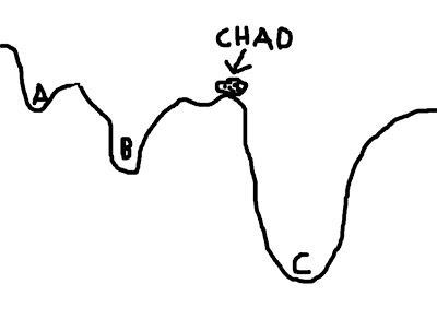
To visualize this concept, imagine a boulder rolling down valleys. The lowest point that the boulder can fall into represents the best solution; the boulder - named Chad - is happiest when he is at the lowest point he can find. However, there are several dips and dells and dales and swales that Chad can roll into, and if he doesn't search around far enough, he may imagine himself to be in the lowest place in the valley - even if that is not necessarily the case. In the picture below, let's say that Chad starts between points A and B; if he looks at the two options, he chooses B, since it is lower, and Chad is therefore happier. However, Chad, in his shortsightedness, has failed to look beyond those two options and descry option C, which in truth is the lowest point of all the valleys.


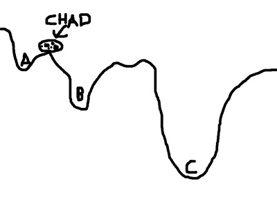
This represents a faulty starting position; and although Chad could extend the range of his search, the range of his gaze, and behold all of the options underneath the pandemonium of the dying sun, this would take far longer. Think of this as corresponding to the search space; expanding this space requires more computing time, which is undesirable.

To mitigate this problem, we can give Chad a hand by placing him in a location where he is more likely to find the optimal solution. For example, let us place Chad closer to C - conceivably, even within C itself - and he will find it much easier to roll his rotund, rocky little body into the soft, warm, womb-like crater of option C, and thus obtain a boulder's beggar's bliss.

(For the mathematically inclined, the contours of the valley represent the cost function; the boulder represents the cost function ratio between the source image and the template image; and each letter (A, B, and C) represents a possible minimum in the cost function.)


As with Chad, so with your anatomical images. It is well for the neuroimager to know that the origin (i.e., coordinates 0,0,0) of both Talairach and MNI space is roughly located at the anterior commissure of the brain; therefore, it behooves you to set the origins of your anatomical images to the anterior commissure as well. The following tutorial will show you how to do this in SPM, where this technique is most important:


Once we have successfully warped our anatomical image to a template space, the reason for coregistration becomes apparent: Since our T2-weighted functional images were in roughly the same space as the anatomical image, we can apply the same warps used on the anatomical image to the functional images. This is where the "Other Images" option comes into play in the SPM interface.


As always, check your registration. Then, check it again. Then, ask someone else to check it. (This is a great way to meet girls.) In particular, check to make sure that the internal structures (such as the ventricles) are properly aligned between the template image and your warped images; matching the internal variability of the template image is much trickier, and therefore much more susceptible to failure - even if the outer boundaries of the brain look as though they match up.


*Actually, it's more accurate to say that it is compressed. However, once I started with the Procrustean thing, I just had to roll with it.
 

Stats Videos (Why do you divide samples by n-1?)

Because FMRI analysis requires a strong statistical background, I've added a couple videos going over the basics of statistical inference, and I use both R and Excel to show the output of certain procedures. In this demo, I go over why the sums of squares of sample populations are divided by n-1; a concept not covered in many statistical textbooks, but an important topic for understanding both statistical inference and where degrees of freedom come from. This isn't a rigorous proof, just a demonstration of why dividing by n-1 is a unbiased estimation of sample variance.