Conjunction Analysis in AFNI


New Haven may have its peccadillos, as do all large cities - drug dealers, panderers, murder-suicides in my apartment complex, dismemberments near the train station, and - most unsettling of all - very un-Midwestern-like rudeness at the UPS Store - but at least the drivers are insane. Possibly this is a kind of mutually assured destruction pact they have with the pedestrians, who are also insane, and as long as everybody acts chaotically enough, some kind of equilibrium is reached. Maybe.

What I'm trying to say, to tie this in with the theme of the blog, is that conjunction analyses in FMRI allow you to determine whether a voxel or group of voxels passes a statistical threshold for two or more contrasts. You could in theory have as many contrasts as you want - there is no limit to the amount and complexity of analyses that researchers will do, which the less-enlightened would call deranged and obsessive, but which those who know better would label creative and unbridled.

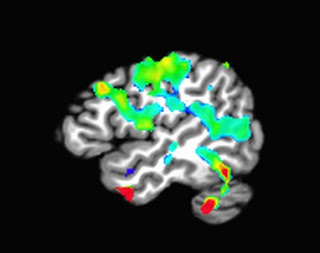
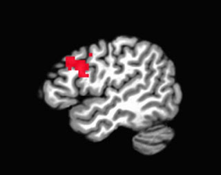
In any case, let's start with the most basic case - a conjunction analysis of two contrasts. If we have one statistical map for Contrast A and another map for Contrast B, we could ask whether there are any voxels common to both A and B. First, we have to ask ourselves, "Why are we in academia?" Once we have caused ourselves enough stress and anxiety asking the question, we are then in the proper frame of mind to move on to the next question, which is, "Which voxels pass a statistical threshold for both contrasts?" You can get a sense of which voxels will show up in the conjunction analysis by simply looking at both contrasts in isolation; in this case, thresholding each by a voxel-wise p-corrected value of 0.01:


Contrast 1

Contrast 2

Conjunction

Note that the heaviest degree of overlap, here around the DLPFC region, is what passes the conjunction analysis.

Assuming that we set a voxel-wise uncorrected threshold of p=0.01, we would have the following code to generate the conjunction map:

3dcalc -prefix conjunction_map -a contrast1 -b contrast2 -expr 'step(a-2.668) + 2*step(b-2.668)'


All you need to fill in is the corresponding contrast maps, as well as your own t-statistic threshold. This will change as a result of the number of subjects in your analysis, but should be relatively stable for large numbers of subjects. When looking at the resulting conjunction map, in this case, you would have three values (or "colors") painted onto the brain: 1 (where contrast 1 passes the threshold), 2 (where contrast 2 passes the threshold), and 3 (where both pass the threshold). You can manipulate the slider bar so that only the number 3 shows, and then use that as a figure for the conjunction analysis.


For more than two contrasts

If you have more than two contrasts you are testing for a conjunction, then modify the above code to include a third map (with the -c option), and multiply the next step function by 4, always going up by a power of 2 as you increase the number of contrasts. For example, with four contrasts:

3dcalc -prefix conjunction_map -a contrast1 -b contrast2 -c contrast 3 -d contrast4 -expr 'step(a-2.668) + 2*step(b-2.668) + 4*step(c-2.668) + 8*step(d-2.668)'


Why is it to the power of 2?

I'll punt on this one and direct you to Gang Chen's page, which has all the information you want, expressed mathematics-style.


Exercises

1. Open up your own AFNI viewer, select two contrasts that you are interested in conjoining, and select an uncorrected p-threshold of 0.05. What would this change in the code above? Why?

2. Imagine the following completely unrealistic scenario: Your adviser is insane, and wants you to do a conjunction analysis of 7 contrasts, which he will probably forget about as soon as you run it. Use the same T-threshold in the code snippet above. How would you write this out?

3. Should you leave your adviser? Why or why not? Create an acrostic spelling out your adviser's name, and use the first letter on each line to spell out a good or bad attribute. Do you have more negative than positive words? What does this tell you about your relationship?
K-Means Analysis with FMRI Data

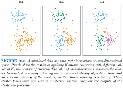
Clustering, or finding subgroups of data, is an important technique in biostatistics, sociology, neuroscience, and dowsing, allowing one to condense what would be a series of complex interaction terms into a straightforward visualization of which observations tend to cluster together. The following graph, taken from the online Introduction to Statistical Learning in R (ISLR), shows this in a two-dimensional space with a random scattering of observations:


Different colors denote different groups, and the number of groups can be decided by the researcher before performing the k-means clustering algorithm. To visualize how these groups are being formed, imagine an "X" being drawn in the center of mass of each cluster; also known as a centroid, this can be thought of as exerting a gravitational pull on nearby data points - those closer to that centroid will "belong" to that cluster, while other data points will be classified as belonging to the other clusters they are closer to.

This can be applied to FMRI data, where several different columns of data extracted from an ROI, representing different regressors, can be assigned to different categories. If, for example, we are looking for only two distinct clusters and we have several different regressors, then a voxel showing high values for half of the regressors but low values for the other regressors may be assigned to cluster 1, while a voxel showing the opposite pattern would be assigned to cluster 2. The label itself is arbitrary, and is interpreted by the researcher.

To do this in Matlab, all you need is a matrix with data values from your regressors extracted from an ROI (or the whole brain, if you want to expand your search). This is then fed into the kmeans function, which takes as arguments the matrix and the number of clusters you wish to partition it into; for example, kmeans(your_matrix, 3).

This will return a vector of numbers classifying a particular row (i.e., a voxel) as belonging to one of the specified clusters. This vector can then be prefixed to a matrix of the x-, y-, and z-coordinates of your search space, and then written into an image for visualizing the results.

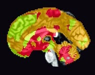
There are a couple of scripts to help out with this: One, createBlankNIFTI.m, which will erase a standardized space image (I suggest a mask output by SPM at its second level) and replace every voxel with zeros, and the other script, createNIFTI.m, will fill in those voxels with your cluster numbers. You should see something like the following (here, I am visualizing it in the AFNI viewer, since it automatically colors in different numbers):

Sample k-means analysis with k=3 clusters.

The functions are pasted below, as well as a couple of explanatory videos.


function createBlankNIFTI(imageFile)

%Note: Make sure that the image is a copy, and retain the original

X = spm_read_vols(spm_vol(imageFile));
X(:,:,:) = 0;
spm_write_vol(spm_vol(imageFile), X);


=================================

function createNIFTI(imageFile, textFile)


hdr = spm_vol(imageFile);
img = spm_read_vols(hdr);

fid = fopen(textFile);
nrows = numel(cell2mat(textscan(fid,'%1c%*[^\n]')));
fclose(fid);

fid = 0;


for i = 1:nrows
    if fid == 0
        fid = fopen(textFile);
    end
    
    Z = fscanf(fid, '%g', 4);
    
    img(Z(2), Z(3), Z(4)) = Z(1);
    spm_write_vol(hdr, img);
end


Dissertation Defense Post-Mortem

A few weeks ago, I mentioned that I had my dissertation defense coming up; understandably, some of you are probably interested in how that went. I'll spare you the disgusting details, and come out and say that I passed, that I made revisions, submitted them about a week and a half ago, and participated in the graduation ceremony in full regalia, which I discarded afterward in the back of a U-Haul truck for immediate transportation to a delousing facility located somewhere on campus. Given that I was sweating like a skunk for nearly three hours (Indiana has quite a few graduates, it turns out), that's probably a wise choice.

For those who need proof that any of this happened, here's a photo:


I believe this conveys everything you need to know. Also, it costs considerably less than paying for the professional photos they took during graduation. Don't get me wrong; the ceremony itself was an incredible spectacle, complete with the ceremonial mace, tams and tassels and gowns of all fabrics and colors, and the president of the university wearing a gigantic medallion that makes even the most flamboyantly attired rapper look like a kindergartener. Even for all that, however, I don't believe it justifies photos at $50 a pop.

Currently I am in Los Angeles, after an extended stint in Vancouver Island visiting strange lands and people, touring the famous Butchart Gardens, and feeding already-overfed sea lions the size of airplane turbines. Then it's back to Minneapolis, Chicago, and finally Bloomington to pack up and leave for the East Coast.

Leave One Subject Out Cross Validation - The Video

Due to the extraordinary popularity of the leave-one-subject-out (LOSO) post I wrote a couple of years ago, and seeing as how I've been using it lately and want to remember how to do it, here is a short eight-minute video on how to do it in SPM. While the method itself is straightforward enough to follow - GLMs are estimated for each group of subjects excluding one subject, and then estimates are extracted from the resulting ROIs for just that subject - the major difficulty is batching it, especially if there are many subjects.

Unfortunately I haven't been able to figure this out satisfactorily; the only advice I can give is that once you have a script that can run your second-level analysis, loop over it while leaving out consecutive subjects for each GLM. This will leave you with the same number of second-level GLMs as there are subjects, and each of these can be used to load up contrasts and observe the resulting clusters from that analysis. Then you extract data from your ROIs for that subject which was left out for the GLM and build up a vector of datapoints for each subject from each GLM, and do t-tests on it, put chocolate sauce on it, eat it, whatever you want. Seriously. Don't tell me I'm the only one who's thought of this.

Once you have your second-level GLM for each subject, I recommend using the following set of commands to get that subject's unbiased data (I feel slightly ridiculous just writing that: "unbiased data"; as though the data gives a rip about anything one way or the other, aside from maybe wanting to be left alone, and just hang out with its friends):

1. Load up your contrast, selecting your uncorrected p-value and cluster size;
2. Click on your ROI and highlight the corresponding coordinates in the Results windown;
3. Find out what the path is to the contrasts for each subject for that second-level contrast by typing "SPM.xY.P"; that will be the template you will alter to get the single subject's data - for example, "/data/myStudy/subject_101/con_0001.img" - and then you can save this to a variable, such as "subject_101_contrast";
4. Average that subject's data across the unbiased ROI (there it is again! I can't get away from it) using something like "mean(spm_get_data(subject_101_contrast, xSPM.XYZ), 2)";
5. Save the resulting value to a vector, and update this for each additional subject.


The Defense


"In 1594, being then seventeen years of age, I finished my courses of philosophy and was struck with the mockery of taking a degree in arts. I therefore thought it more profitable to examine myself and I perceived that I really knew nothing worth knowing. I had only to talk and wrangle and therefore refused the title of master of arts, there being nothing sound or true that I was a master of. I turned my thoughts to medicine and learned the emptiness of books. I went abroad and found everywhere the same deep-rooted ignorance."

-Van Helmont (1648)


"The new degree of Bachelor of Science does not guarantee that the holder knows any science. It does guarantee that he does not know any Latin."

-Dean Briggs of Harvard College (c. 1900) 


When I was a young man I read Nabokov's The Defense, which, I think, was about a dissertation defense and the protagonist Luzhin's (rhymes with illusions) ensuing mental breakdown. I can't remember that much about it; but the point is that a dissertation defense - to judge from the blogs and article posts written by calm, rational, well-balanced academics without an axe to grind, and who would never, ever exaggerate their experience just for the sake of looking as though they struggle and suffer far more than everybody else - is one of the most arduous, intense, soulcrushing, backbreaking, ballbusting, brutal experiences imaginable, possibly only equaled by 9/11, the entire history of slavery, and the siege of Stalingrad combined. Those who survive it are, somehow, of a different order.

The date has been set; and just like a real date, it will involve awkward stares, nervous laughter, and the sense that you're not quite being listened to - but without the hanky-panky at the end. The defense is in three days, and part of me knows that most of it is done already; having prepared myself well, and having selected a panel of four arbiters who, to the best of my knowledge, when placed in the same room will not attempt to eat each other. ("Oh come on, just a nibble?" "NEIN!")

Wish me luck, comrades. During the defense, the following will be playing in my head:


Slice Analysis of FMRI Data with SPM


Slice analysis is a simple procedure - first you take a jar of peanut butter and a jar of Nutella, and then use a spoon to take some Nutella and then use the same spoon to mix it with the peanut butter. Eat and repeat until you go into insulin shock, and then...

No, wait! I was describing my midnight snack. The actual slice analysis method, although less delicious, is infinitely more helpful in determining regional dissociations of activity, as well as avoiding diabetes. (Although who says they can't both be done at the same time?)

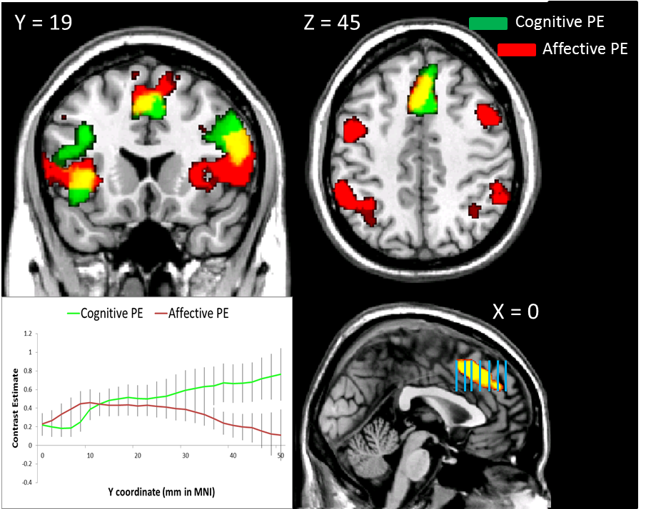
The first step is to extract contrast estimates for each slice from a region of interest (ROI, also pronounced "ROY") and then average across all the voxels in that slice for the subject. Of course, there is no way you would be able to do this step on your own, so we need to copy someone else's code from the Internet and adapt it to our needs; one of John Ashburner's code snippets (#23, found here) is a good template to start with. Here is my adaptation:


rootdir = '/data/drill/space10/PainStudy/fmri/'; %Change these to reflect your directory structure
glmdir = '/RESULTS/model_RTreg/'; %Path to SPM.mat and mask files

subjects = [202:209 211:215 217 219 220:222 224:227 229 230 232 233];
%subjects = 202:203;

Conditions.names = {'stroopSurpriseConStats', 'painSurpriseConStats'}; %Replace with your own conditions
Masks = {'stroopSurpriseMask.img', 'painSurpriseMask.img'}; %Replace with your own masks; should be the product of a binary ROI multiplied by your contrast of interest
Conditions.Contrasts = {'', ''};

ConStats = [];
Condition1 = [];
Condition2 = [];

for i=subjects
    
    cd([rootdir num2str(i) glmdir])
    outputPath = [rootdir num2str(i) glmdir]; %Should contain both SPM.mat file and mask files
    
    for maskIdx = 1:length(Masks)
      
    P = [outputPath Masks{(maskIdx)}];

    V=spm_vol(P);

    tmp2 = [];
    
     [x,y,z] = ndgrid(1:V.dim(1),1:V.dim(2),0);
     for i=1:V.dim(3),
       z   = z + 1;
       tmp = spm_sample_vol(V,x,y,z,0);
       msk = find(tmp~=0 & isfinite(tmp));
       if ~isempty(msk),
         tmp = tmp(msk);
         xyz1=[x(msk)'; y(msk)'; z(msk)'; ones(1,length(msk))];
         xyzt=V.mat(1:3,:)*xyz1;
         for j=1:length(tmp),
           tmp2 = [tmp2; xyzt(1,j), xyzt(2,j), xyzt(3,j), tmp(j)];
         end;
       end;
     end;

         xyzStats = sortrows(tmp2,2); %Sort relative to second column (Y column); 1 = X, 3 = Z
         minY = min(xyzStats(:,2));
         maxY = max(xyzStats(:,2));

         ConStats = [];

     for idx = minY:2:maxY
         x = find(xyzStats(:,2)==idx); %Go in increments of 2, since most images are warped to this dimension; however, change if resolution is different
         ConStats = [ConStats; mean(xyzStats(min(x):max(x),4))];
     end

    if maskIdx == 1
        Condition1 = [ConStats Condition1];
    elseif maskIdx == 2
        Condition2 = [ConStats Condition2];
    end

    end
end

Conditions.Contrasts{1} = Condition1;
Conditions.Contrasts{2} = Condition2;


This script assumes that there are only two conditions; more can be added, but care should be taken to reflect this, especially with the if/else statement near the end of the script. I could refine it to work with any amount of conditions, but that would require effort and talent.

Once these contrasts are loaded into your structure, you can then put them in an Excel spreadsheet or any other program that will allow you to format and save the contrasts in a tab-delimited text format. The goal is to prepare them for analysis in R, where you can test for main effects and interactions across the ROI for your contrasts. In Excel, I like to format it in the following four-column format:


Subject Condition Position  Contrast
202 Stroop 0 -0.791985669
202 Stroop 2 -0.558366941
202 Stroop 4 -0.338829942
202 Pain 0 0.17158524
202 Pain 2 0.267789503
202 Pain 4 0.192473782
203 Stroop 0 0.596162455
203 Stroop 2 0.44917655
203 Stroop 4 0.410870348
203 Pain 0 0.722974284
203 Pain 2 0.871030304
203 Pain 4 1.045700207


And so on, depending on how many subjects, conditions, and slices you have. (Note here that I have position in millimeters from the origin in the y-direction; this will depend on your standardized space resolution, which in this case is 2mm per slice.)

Once you export that to a tab-delimited text file, you can then read it into R and analyze it with code like the following:

setwd("~/Desktop")
x = read.table("SliceAnalysis.txt", header=TRUE)
x$Subject <- as.factor="" font="" ubject="" x="">
aov.x = aov(Contrast~(Condition*Position)+Error(Subject/(Condition*Position)),x)
summary(aov.x)
interaction.plot(x$Position, x$Condition, x$Contrast)


This will output statistics for main effects and interactions, as well as plotting the contrasts against each other as a function of position.

That's it! Enjoy your slices, crack open some jars of sugary products, and have some wild times!


Automating SPM Contrasts

Manually typing in contrasts in SPM is a grueling process that can have a wide array of unpleasant side effects, including diplopia, lumbago, carpal tunnel syndrome, psychosis, violent auditory and visual hallucinations, hives, and dry mouth. These symptoms are only compounded by the number of regressors in your model, and the number of subjects in your study.

Fortunately, there is a simply way to automate all of this - provided that each subject has the same number of runs, and that the regressors in each run are structured the same way. If they are, though, the following approach will work.

First, open up SPM and click on the TASKS button in the upper right corner of the Graphics window. The button is marked "TASKS" in capital letters, because they really, really want you to use this thing, and mitigate all of the damage and harm in your life caused by doing things manually. You then select the Stats menu, then Contrast Manager. The options from there are straightforward, similar to what you would do when opening up the Results section from the GUI and typing in contrasts manually.

When specifying the contrast vector, take note of how many runs there are per subject. This is because we want to take the average parameter estimate for each regressor we are considering; one can imagine a scenario where one of the regressors occurs in every run, but the other regressor only happens in a subset of runs, and this more or less puts them on equal footing. In addition, comparing the average parameter or contrast estimate across subjects is easier to interpret.

Once you have the settings to your satisfaction, save it out as a .mat file - for example, 'RunContrasts.mat'. This can then be loaded from the command line:

load('RunContrasts')

Which will put a structure called "jobs" in your workspace, which contains all of the code needed to run a first-level contrast. The only part of it we need to change when looping over subjects is the spmmat field, which can be done with code like the following:

subjList=[207 208]; %And so on, including however many subjects you want

for subj=subjList

    jobs{1}.stats{1}.con.spmmat =     {['/data/hammer/space4/MultiOutcome2/fmri/' num2str(subj) '/RESULTS/model_multiSess/SPM.mat']} %This could be modified so that the path is a variable reflecting where you put your SPM.mat file
    spm_jobman('run', jobs)

end

This is demonstrated in the following pair of videos; the first, showing the general setup, and the second showing the execution from the command line.


Important Announcement from Andy's Brain Blog

Even though I assume that the readers of this blog are a small circle of loyal fanatics willing to keep checking in on this site even after I haven't posted for months, and although I have generally treated them with the same degree of interest I would give a Tupperware container filled with armpit hair, even they are entitled to a video update that features me sitting smugly with a cheesy rictus pasted on my face as I list off several of my undeserved accomplishments, as well as giving a thorough explanation for my long absence, and why I haven't posted any truly useful information in about a year. (Hint: It starts with a "d", and rhymes with "missertation.")

Well, the wait is over! Here it is, complete with a new logo and piano music looping softly in the background that kind of sounds like Coldplay!


For those of you who don't have the patience to sit through the video (although you might learn a thing or two about drawing ROIs with fslmaths, which I may or may not have covered a while back), here are the bullet points:


  • After several long months, I have finished my dissertation. It has been proofread, edited, converted into a PDF, and sent out to my committee where it will be promptly filed away and only skimmed through furiously on the day of my defense, where I will be grilled on tough issues such as why my Acknowledgements section includes names like Jake & Amir.
  • A few months ago I was offered, and I accepted, a postdoctoral position at Haskins Laboratories at Yale. (Although technically an independent, private research institution, it includes the name Yale in its web address, so whenever anybody asks where I will be working, I just say "Yale." This has the double effect of being deliberately misleading and making me seem far more intelligent than I am.) I recently traveled out there to meet the people I would be working with, took a tour of the lab, walked around New Haven, sang karaoke, and purchased a shotgun and a Rottweiler for personal safety reasons. Well, the Rottweiler more because I'll be pretty lonely once I get out there, and I need someone to talk to.
  • When I looked at the amount of money I would be paid for this new position, I couldn't believe it. Then when I looked at the amount of money I would be paying for rent, transportation, excess nosehair taxes (only in a state like Connecticut), shotgun ammunition, and dog food, I also couldn't believe it. Bottom line is, my finances will not change considerably once I move.
  • A new logo for the site has been designed by loyal fanatic reader Kyle Dunovan who made it out of the goodness of his heart, and possibly because he is banking on bigtime royalties once we set up an online shop with coffee mugs and t-shirts. In any case, I think it perfectly captures the vibe of the blog - stylish, cool, sleek, sophisticated, red, blue, green, and Greek.
  • Lastly, I promise - for real, this time, unlike all of those other times - to be posting some cool new techniques and tools you can use, such as slice analysis, leave-one-out analysis, and k-means clustering (as soon as I figure that last one out). Once I move to Connecticut the focus will probably shift to more big data techniques, with a renewed emphasis on online databases, similar to previous posts using the ABIDE dataset.
  • I hope to catch up on some major backlogging with emails, both on the blog and on the Youtube channel. However, I can't promise that I will get to all of them (and there are a LOT). One heartening development is that more readers are commenting on other questions and posts, and helping each other out. I hope that the community continues to grow like this, which will be further bonded through coffee mugs and t-shirts with the brain blog logo on it.

Spain


Fellow brainbloggers,

Like a neglectful parent, I have been away far too long - although I did leave twenty dollars on the kitchen table for you to order pizza - and while I could recite the usual litany of excuses, including job searching, teaching, writing papers, sorting the recycling, learning glassblowing, and recovering from gout, none of those warrants such an excessive absence; especially given the supportive, heartwarming messages I have received from some of you describing how the blog has helped save time, money, and, I like to think, relationships. Maybe. If you've learned nothing else, just remember that the most important part of a relationship is winning every argument.

However, as the end of my graduate school years comes closer, I have had to make difficult decisions resulting in the abandonment of the mistress of my youth, blogging, for the wife of mine age, dissertation writing. I never thought I would end up like all the others at this stage, finding myself using all of my free time to work on my dissertation. Partly it is because using the excuse of working on your dissertation is incredibly effective at getting out of any undesirable obligations. For example:


Injured Friend: Andy, I need to stanch the bleeding caused by a freak accident involving a pair of nosehair trimmers. Please help.
Me: You know I would, but I have to work on my dissertation.
Injured Friend: Of course; how selfish of me.

Girlfriend: Andy, we've been in a long-distance relationship for three years now, but during that time I have only seen you once on Skype - and that was just to tell me the joke about who they found in Jeffrey Dahmer's freezer*. I need more commitment from you.
Me: Sorry, Schmoopy, but I have to work on my dissertation.
Girlfriend: Whenever you say "I have to work on my dissertation," you sound so incredibly confident, productive, and sexy. I completely understand, and apologize for any inconvenience I may have caused.

Advisor: Andy, you need to spend less time screwing around, and more time working on your dissertation.
Me: Maybe, but I should probably work on my dissertation instead.
Advisor: Holy mackerel, you need to get on that.


The manifest absurdity of such statements doesn't seem to strike anybody as particularly odd - after all, you are slogging away for long hours on something productive and good, and not, say, out in the streets mugging anybody, or committing cyberterrorism - and this fills many graduate students with a satisfying sense of self-righteousness.

In any case, if you have written regarding any questions or issues, I will get to it eventually - there is a bit of a backlog at the moment, and I've had to do some triage. Although you should probably know that, again like a neglectful parent, I will be going to Spain for the holidays. That's right, I said Spain. And although I realize it may not always be the wisest thing to advertise when I am away from my apartment, please don't break into it while I'm gone. (Although, if you do, there are hotpockets in the freezer. Just saying.)


*Ben and Jerry.