Youtube Music Channel

One of my hobbies is playing piano, and recently I bought the equipment to record sound from my electric piano. I own a Yamaha CLP-320 series, which has been an excellent piano and has held up remarkably well for the past three years.

The first recording uploaded from this piano is a nocturne by Chopin in B-flat minor,  opus 9, #1. I have had it in my repertoire for quite a while now, and it still remains my favorite nocturne out of all of them. I plan to upload more recordings with some regularity (e.g., every week or two), so be sure to check out the channel often to see what's new. Subscribing (or even just "liking") is a great way to help me out.

One feature of my videos is annotations which highlight certain interesting parts of the piece, such as important key modulations, any historical background that might be significant, and so on. I also think it looks cool when Chopin spits facts about his music. My goal is for it to be edifying rather than distracting; time will tell whether the public likes it or not.

Anyway, here's a link to the video. Enjoy!

[Edit 07.08.2012]: I removed the annotations, because I eventually found them distracting. Any notes will be placed in the "Description" box, as soon as I convince the recording companies that this indeed my own original work, and not a copy.


Region of Interest Analysis


Before we get down to regions of interest, a few words about the recent heat wave: It's taken a toll. The past few days I've walked out the door and straight into a slow broil, that great yellowish orb pasted in the cloudless sky like a sticker, beating down waves of heat that saps all the energy out of your muscles. You try to get started with a couple miles down the country roads, crenelated spires of heat radiating from the blacktop, a thin rime of salt and dust coating every inch of your skin, and realize the only sound in this inferno is the soles of your shoes slapping the cracked asphalt. Out here, even the dogs have given up barking. Any grass unprotected by the shade of nearby trees has withered and died, entire lawns turned into fields of dry, yellow, lifeless straw. Flensed remains of dogs and cattle and unlucky travelers lie in the street, bones bleached by the sun, eyeless sockets gazing skyward like the expired votaries of some angry sun god.

In short, it's been pretty brutal.

Regions of Interest

Region of Interest (ROI) analysis in neuroimaging refers to selecting a cluster of voxels or brain region a priori (or, also very common, a posteriori) when investigating a region for effects. This can be done either by creating a small search space (typically a sphere with a radius of N voxels), or based on anatomical atlases available through programs like SPM or downloadable from web. ROI analysis has the advantage of mitigating the fiendish multiple comparisons problem, in which a search space of potentially hundreds of thousands of voxels is reduced to a smaller, more tractable area, thus reducing overly stringent multiple comparisons correction thresholds. At first glance this makes sense, given that you may not be interested in a whole brain analysis (i.e., searching for activation in every single voxel in the entire volume); however, it can also be abused to carry out confirmatory analyses after you have already determined where a cluster of activation is.

Simple example: You carry out a whole brain analysis, and find a cluster of fifty voxels extending over the superior frontal sulcus. This is not a large enough cluster extent to pass cluster correction at the whole brain level, but you go ahead anyway and perform an additional ROI analysis focused on the center of the cluster. There are not any real safeguards against this measure, as it is impossible to know what the researcher had in mind when they conducted the test. For instance, what if an investigator happened to simply make a mistake and see the results of a whole brain analysis before doing an ROI analysis? Pretend that he didn't see them? These are questions which may be addressed in a future post about a Bayesian approach to fMRI, but for now, be aware that there exists significant potential for misuse of this technique.

Additional Considerations


Non-Independence
Colloquially known as "double-dipping," non-independence has become an increasingly important issue over the years as ROI analyses have become more common (see Kriegeskorte et al, 2009, 2010).  In order to avoid biasing an ROI toward certain regressors, it is essential that the ROI and the contrast of interest share no common regressors. Consider a hypothetical experiment with three regressors: A, B, and C.  The contrast A-B is used to define an ROI, and the experimenter then decides to test the contrast of A-C within this ROI.  As this ROI is already biased toward voxels that are more active in response to regressor A, this is a biased contrast to conduct. This is not endemic only to fMRI data, but applies to any other statistical comparison where bias is a potential issue.

Correction for Multiple ROI Analyses
Ideally, each ROI analysis should be treated as an independent test, and should be corrected for multiple comparisons.  That is, assuming that an investigator is agnostic about where the activation is to be found, the alpha threshold for determining significance should be divided by the amount of tests conducted.  While this is probably rarely done, it is good practice to have a priori hypotheses about where activation is to be found in order to avoid these issues of multiple comparisons.

ROI Analysis in AFNI

Within AFNI, there exists a useful program called 3dUndump which requires x, y, and z coordinates (in millimeters), radius size of the sphere, and the master dataset where the sphere will be applied. A typical command looks like:

3dUndump -prefix (OutputDataset) -master (MasterDataset) -srad (Radius of Sphere, in mm) -xyz (X, Y, and Z coordinates of sphere)


One thing to keep in mind is the orientation of the master dataset. For example, the standard template that AFNI warps has a positive to negative gradient when going from posterior to anterior; in other words, values in the Y-direction will be negative when moving forward of the anterior commissure. Thus, it is important to note the space and orientation of the coordinates off of which you are basing your ROI, and make sure it matches up with the orientation of the dataset you are applying the ROI to. In short, look at your data after you have generated the ROI to make sure that it looks reasonable.


The following is a short Python wrapper I made for 3dUndump. Those already familiar with using 3dUndump may not find much use in it, but for me, having an interactive prompt is useful:


#!usr/bin/env python


import os
import math
import sys


#Read in Raw user input, assign to variables
print("MakeSpheres.py")
print("Created by Andrew Jahn, Indiana University 03.14.2012")
prefix = raw_input("Please enter the output filename of the sphere: ")
master = raw_input("Please enter name of master dataset (e.g., anat_final.+tlrc): ")
rad = raw_input("Please enter radius of sphere (in mm): ")
xCoord = raw_input("Please enter x coordinate of sphere (MNI): ")
yCoord = raw_input("Please enter y coordinate of sphere (MNI): ")
zCoord = raw_input("Please enter z coordinate of sphere (MNI): ")


#Make string of coordinates (e.g., 0 36 12)
xyzString = xCoord + " " + yCoord + " " + zCoord
printXYZString = 'echo ' + xyzString + ' > sphere_' + rad + 'mm_'+xCoord+'_'+yCoord+'_'+zCoord+'.txt'
os.system(printXYZString) #prints xyzstring to filename given above


#Will need sphere file in this format for makeSpheres function
xyzFile = 'sphere_' + rad + 'mm_'+xCoord+'_'+yCoord+'_'+zCoord+'.txt'


def makeSpheres(prefix, master, rad, xyz ):
cmdString = '3dUndump -prefix '+prefix+ ' -master '+master+' -srad '+rad+' -xyz '+xyz 
os.system(cmdString)
return


makeSpheres(prefix=prefix, master=master, rad=rad, xyz=xyzFile)


Which will generate something like this (Based on a 5mm sphere centered on coordinates 0, 30, 20):


Beta values, time course information, etc., can then be extracted from within this restricted region.

ROI Analysis in SPM (Functional ROIs)

This next example will focus on how to do ROI analysis in SPM through MarsBar, a toolbox available here if you don't already have it installed. In addition to walking through ROI analysis in SPM, this will also serve as a guide to creating functional ROIs. Functional ROIs are based on results from other contrasts or interactions, which ideally should be independent of the test to be investigated within that ROI; else, you run the risk of double-dipping (see the "Non-Independence" section above).

After installation, you should see Marsbar as an option in the SPM toolbox dropdown menu:

1. Extract ROIs

After installing Marsbar, select it from the toolbox dropdown menu.  After Marsbar boots up, click on the menu “ROI Definition”.  Select “Get SPM clusters”.


This will prompt the user to supply an SPM.mat file containing the contrast of interest.  Select the SPM.mat file that you want, and click “Done”.

Select the contrast of interest just as you would when visualizing any other contrast in SPM.  Select the appropriate contrast and the threshold criteria that you want.


When your SPM appears on the template brain, navigate to the cluster you wish to extract, and click “current cluster” from the menu, underneath “p-value”.  Highlight the cluster you want in the SPM Results table.  The highlighted cluster should turn red after you select it.


Navigate back to the SPM results menu, and click on “Write ROIs”.  This option will only be available if you have highlighted a clutter.  Click on “Write one cluster”.  You can enter your description and label for the ROI; leaving these as default is fine.  Select an appropriate name for your ROI, and save it to an appropriate folder.


2. Export ROI

Next, you will need to convert your ROI from a .mat file to an image file (e.g., .nii or .img format).  Select “ROI Definition” from the Marsbar menu and then “Export”.


You will then be presented with an option for where to save the ROI. 


Select the ROI you want to export, and click Done.  Select the directory where you wish to output the image.  You should now see the ROI you exported, with a .nii extension.

3. ROI Analysis

You can now use your saved image for an ROI analysis.  Boot up the Results menu as you would to normally look at a contrast, but when prompted for “ROI Analysis?”, select “Yes”. You can select your ROI from the “Saved File” option; alternatively, you can mask activity based on atlas parcellations by selecting the “Atlas” option.


The constriction of search space will mean fewer multiple comparisons need to be corrected for, and thus increases the statistical power of your contrast.


Summer Music Festival

For me, one of the major draws of Indiana University - besides its neuroimaging program - was the presence of the Jacobs School of Music, one of the best conservatories in the world. I had studied piano as a kid and have continued to keep it up as a hobby, so for me, a music school within spitting distance from my apartment was a major attraction.

Last summer the Jacobs School began a summer music festival, where nearly every night for the entire summer term there are musical performances. Solo piano recitals, string quartets and chamber music, and symphonic works are performed continuously, with soloists and music ensembles traveling from all over the world to play here. Tickets are six dollars for students, and piano recitals are free. For a piano addict like myself, with Carnegie Hall-caliber performances going on all day, every day - this is bliss.

One of the themes this summer is a complete cycle of the sixteen Beethoven string quartets. I had heard a few of the earlier works, but had put off listening to the later quartets because I didn't feel quite ready for them yet - many of them are tremendously difficult to listen to, approaching colossal lengths and levels of complexity that are almost impenetrable. Although immensely rewarding, this is not the same as saying it is a pleasurable experience.

However, I decided to go through with it anyway, and on Sunday I witnessed a performance of one of the last works ever composed by Ludwig van, the string quartet in B-flat major, opus 130. Back when it first premiered Beethoven had composed a gigantic, dissonant double fugue as the final movement, stretching the entire performance to almost an hour. It was met with resistance from the public and critics alike, and Beethoven's publisher convinced him to substitute a lighter, more accessible ending. Beethoven relented (begrudgingly), and published the fugue separately, entitling the work "Große Fugue", which means Great Fugue, or Grand Fugue. Because of its tremendous duration and emotional scope, the work has since been frequently performed on its own as an example of Beethoven's late style and contrapuntal daring.

Which is why I was surprised that, before the performance, the second violinist addressed the audience and informed us that contrary to what was on the program, they were going to play the work with the original fugue ending. Holy crap, I thought: It is on.

The next hour was intense, with the titanic opening, middle, and ending movements flanked by smaller, intense interludes, an architecture that characterized much of Beethoven's late output. The Fugue, as expected, was gigantic, and the musicians were sawing away at their instruments, squeezing the lemon so to speak, and somehow sustaining the whole thing without letting it degrade into complete chaos. I was extremely impressed, and recommend that anyone who has the chance should see these guys live, or at least listen to one of their CDs.


During the performance, one interesting musical reference I noticed was a theme consisting of a leap followed by a trill - a similar theme that opens the finale of Beethoven's Hammerklavier Sonata, also in B-flat major, and also ending with a fugue on acid. The jump in that work is much larger and more dramatic - almost a tenth, I think - but the similarity was striking. In the following video, listen to the trill theme starting around 7:45, and then compare with the opening of the Hammerklavier fugue. And then you might as well watch the whole thing, because Valentina Lisitsa's spidery, ethereal hands are beautiful to watch.


In all, it was a heroic performance, and I am looking forward to completing the cycle over the next couple of weeks.

The next couple of days will see a return to the cog neuro side of things, since it has been a while since I've written about that. I have a new program written for building regions of interest in AFNI, as well as some FSL and UNIX tutorials which should be online soon. Stay tuned!

Grandma's Marathon Postmortem


[Note: I don't have any personal race photos up yet; they should arrive in the next few days]


Finally back in Bloomington, after my standard sixteen-hour Megabus trip from Minnesota to Indiana, with a brief layover in Chicago to see The Bean. I had a successful run at Grandma's, almost six minutes faster than my previous marathon, which far exceeded my expectations going into it.

Both for any interested readers, and for my own personal use to see what I did leading up to and during race day, I've broken down the experience into segments:

1. Base Phase

I rebooted my training over winter break coming back from a brief running furlough, after feeling sapped from the Chicago Marathon. I began running around Christmas, starting with about 30 miles a week and building up to about 50 miles a week, but rarely going above that for some months. Now that I look back on it, this really isn't much of a base phase at all, at least according to the books I've read and runners I've talked to; but that was the way it worked out with graduate school and my other obligations.

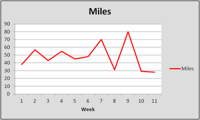
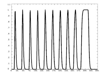
Here are the miles per week, for eleven weeks, leading up to Grandma's:

Week 1: 38
Week 2: 57
Week 3: 43
Week 4: 55
Week 5: 45
Week 6: 48
Week 7: 70
Week 8: 31
Week 9: 80
Week 10: 29
Race Week: 28 (not including the marathon)


2. Workouts

The only workouts I do are 1) Long runs, typically 20-25 miles; and 2) Tempo runs, usually 12-16 miles at just above (i.e., slower than) threshold pace, which for me is around 5:40-5:50 a mile. That's it. I don't do any speedwork or interval training, which is a huge weakness for me; if I ever go under my lactate threshold too early, I crash hard. It has probably been about two years since I did a real interval workout, and I should probably get back to doing those sometime. The only thing is, I have never gotten injured or felt fatigued for days after doing a tempo run, whereas I would get stale and injured rather easily doing interval and speed workouts. In all likelihood I was doing them at a higher intensity than I should have when I was doing them.

3. TV Shows

The only TV show that I really watch right now is Breaking Bad, and the new season doesn't begin until July 15th. So, I don't have much to say about that right now.

4. Race Day

In the week leading up to the race, I was checking the weather reports compulsively. The weather for events like this can be fickle down to the hour, and the evening before the race I discussed race strategy with my dad. He said that in conditions like these, I would be wise to go out conservative and run the first couple of miles in the 6:00 range. It seemed like a sound plan, considering that I had done a small tune-up run the day before in what I assumed would be similar conditions, and the humidity got to me pretty quickly. In short, I expected to run about the same time I did at the Twin Cities marathon in 2010.

The morning of the race, the weather outside was cooler and drier than I expected, with a refreshing breeze coming in from Lake Superior. I boarded the bus and began the long drive to the start line, which really makes you realize how far you have to run to get back. I sat next to some guy who looked intense and pissed off and who I knew wouldn't talk to me and started pounding water.

At the starting line everything was warm and cheerful and sun-soaked and participants began lining up according to times posted next to the corrals. I talked to some old-timer who had done the race every single year, who told me about the good old days and how there used to only be ten port-a-johns, and how everyone would go to that ditch over yonder where the grassy slopes would turn slick and putrid. I said that sounded disgusting, and quickly walked over to my corral to escape.

Miles 1-6

At the start of the race, I decided to just go out on feel and take it from there. The first mile was quickly over, and at the mile marker my watch read: 5:42. I thought that I might be getting sucked out into a faster pace than I anticipated, but since I was feeling solid, I thought I would keep the same effort, if not back off a little bit, and then see what would happen. To my surprise, the mile splits got progressively faster: 5:39, 5:36, 5:37, 5:34, 5:33. I hit the 10k in about 34:54 and started to have flashbacks to Chicago last fall, where I went out at a similar pace and blew up just over halfway through the race. However, the weather seemed to be holding up, and actually getting better, instead of getting hotter and more humid. At this point my body was still feeling fine so I settled in and chose to maintain the same effort for the next few miles.

Miles 7-13

Things proceeded as expected, with a 5:34, 5:38, and 5:35 bringing me to mile 9. I saw my parents again at this point, both looking surprised that I had come through this checkpoint several minutes faster than planned. Although I knew it was fast, I didn't really care; at this point the weather had become decidedly drier than it was at the start of the race, the crowd was amping up the energy, and I was feeling bulletproof. It was also right about this time that I started feeling a twinge in my upper left quadricep.

Shit.

I had been having problems with this area for the past year, but for the last month things had settled down and it hadn't prevented my completing any workouts for the past few weeks. Still, it was a huge question mark going into the race, and with over sixteen miles to go, it could put me in the hurt locker and possibly force me to pull out of the race. I knew from experience that slowing down wouldn't help it so I continued at the same pace, hoping that it might go away.

5:28, 5:40, 5:37, 5:44. Although I was able to hold the same pace, the quadricep was getting noticeably worse, and began to affect my stride. I ignored it as best I could, trying instead to focus on the fact that I had come through the half in 1:13:40, which was close to a personal best and almost identical to what I had done at Chicago. I kept going, prepared to drop out at the next checkpoint if my leg continued to get worse.

Miles 14-20

The next couple of miles were quicker, with a 5:28 and 5:38 thanks to a gradual downhill during that section of the race. As I ran by the fifteen-mile marker, I began to notice that my quadricep was improving. The next pair of miles were 5:42, 5:42. At this point there was no mistaking it: The pain had completely disappeared, something that has never happened to me before. Sometimes I am able to run through mild injuries, but for them to recover during the course of a race, was new to me.

In any case, I didn't dwell on it. The next few miles flew by in 5:48, 5:38, and 5:55, and I knew that past the twenty-mile mark things were going to get ugly.

Miles 21-26.2

As we began our descent into the outskirts of Duluth, the crowds became larger and more frequent, clusters of bystanders serried together with all sorts of noisemakers and signs that sometimes had my name on them, although they were meant for someone else. At every aid station I doused myself with water and rubbed cool sponges over my  face and shoulders, trying not to overheat. 5:57, 5:56. However, even though I was slowing way down, mentally I was still with it and able to focus. We had entered the residential neighborhoods, and the isolated bands of people had blended together into one long, continuous stream of spectators lining both sides of the road. I made every attempt to avoid the cracks in the street, sensing that if I made an uneven step, I might fall flat on my face.

5:55. Good, not slowing down too much. Still a few miles out, but from here I can see the promontory where the finish line is. At least, that's where I think it is. If that's not it, I'm screwed. Why are these morons trying to high-five me? Get the hell out of my way, junior. Just up and over this bridge. Do they really have to make them this steep? The clown who designed these bridges should be dragged into the street and shot. 6:03. I was hoping I wouldn't have any of those. I can still reel in a few of these people in front of me. This guy here is hurting bad; I would feel sorry for him, but at the same time it's such a rush to pass people when they are in a world of pain; almost like a little Christmas present each time it happens. 6:03 again. Oof. We've made another turn; things are getting weird. Where's the finish? Where am I? What's my favorite food? I can't remember. This downhill is steep as a mother, and I don't know if those muscles in my thighs serving as shock pads can take much more of this. Legs are burning, arms are going numb, lips are cracked and salty. One more mile to go here; just don't throw up and don't lose control of your bowels in front of the cameras and you're golden. 6:11. Whatever. There's the finish line; finally. Wave to the crowd; that's right, cheer me on, dammit! Almost there...and...done.

YES.


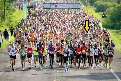
Artist's rendering of what I looked like at the finish

29th overall, with a time of 2:30:23. I staggered around the finish area, elated and exhausted, starting to feeling the numbness creep into my muscles. For the next few days I had soreness throughout my entire body, but no hematuria, which is a W in my book.

More results can be found here, as well as a summary page here with my splits and a video showcasing my raw masculinity as I cross the finish line.

Next marathon will be in Milwaukee in October, and I'll be sure to give some running updates as the summer progresses.

Grandma's! I am coming for you!

Hey all, I will be gone until next Tuesday for a brief trip back to Minnesota to see some relatives and race Grandma's marathon. Conditions are supposed to be in the upper 50s at racetime, partly cloudy, tailwind of 9mph, and a slight net downhill, which should be ideal for running a personal best.


According to my training logs, VO2 max, past running history, and a Ouija board, I should be somewhere in the neighborhood of running a 2:32:00 (roughly 5:48/mile). You can track my progress here on the Grandma's Marathon website (first name: Andrew; last name: Jahn).

I'll be posting a post-race analysis sometime early next week. Wish me luck!

Smoothing in AFNI

What Smoothing Is


Smoothing, the process of introducing spatial correlation into your data by averaging across nearby data points (in fMRI datasets, nearby voxels) is an essential step in any preprocessing stream. Traditionally, smoothing applies a Gaussian filter to average signal over nearby voxels in order to summate any signal that is present, while attenuating and cancelling out noise. This step also has the advantage of spreading signal over brain areas that have some variation across subjects, leading to increased signal-to-noise ratio over larger cortical areas at the loss of some spatial specificity. Lastly, smoothing mitigates the fiendish multiple comparisons problem, since voxels are not truly independent in the first place (neither are timepoints, but more on this at a later time).

Before (left) and after (right) smoothing. Note that there is much more spatial detail in the image before smoothing is applied.


Usually this smoothing step is taken care of by your fMRI software analysis package's built-in smoothing program, but something I learned back at the AFNI bootcamp is that images coming off the scanner are already smoothed, i.e., there is already some inherent spatial correlation in the data. This makes sense, given that functional imaging datasets are acquired at relatively low resolution, and that voxels with a given intensity will most likely be immediately surrounded by other voxels with similar intensities. In the above image on the left which has not been smoothed, voxels that are brighter tend to cluster together, while voxels that are darker tend to cluster together. This spatial correlation will be increased with any additional step requiring spatial interpolation, including coregistration (aligning all volumes in a run to a reference volume), normalization (warping an image to a template space), and smoothing.


Smoothing Programs in AFNI: 3dmerge and 3dBlurToFWHM


In the good old days, the staple program for blurring in AFNI was 3dmerge with the -blur option. Since 2006, there has been a new program, 3dBlurToFWHM, which estimates the smoothness of the dataset, and attempts to smooth only to specified blur amounts in the x, y, and z directions. (Another thing I didn't recognize, in my callow youth, was that there can indeed be different smoothness amounts along the axes of your dataset, which in turn should be accounted for by your smoothing algorithm.) 3dmerge will add on the specified smoothness to whatever smoothness is already present in the data, so the actual smoothness of the data is not what is specified on the command line with 3dmerge. For example, if 3dmerge with a 6mm Full-Width at Half-Maximum (FWHM) is applied to a dataset that already has smoothness of about 3mm in the x, y, and z directions, the resulting smoothness will be about 8-9mm. (This example, similar to many simulations carried out in the lab, is not a purely linear addition, but is relatively close.)


3dBlurToFWHM, on the other hand, will begin with estimating the smoothness of your dataset, and then iteratively blur (i.e., smooth) the data until it reaches the desired level of smoothness in the x, y, and z directions. These can be specified separately, but often it is more useful to use the same value for all three. For example, the following command will blur a dataset until it reaches approximately 6mm of smoothness in each direction:

3dBlurToFWHM -FWHM 6 -automask -prefix outputDataset -input inputDataset

Applying this to a dataset that has been coregistered and normalized will produce output that looks like this:


Note that the first set of numbers highlighted in red are the estimates produced by 3dBlurToFWHM, and the last set of numbers of red are estimates from a separate program, 3dFWHMx. The reason for the discrepancy is that 3dBlurToFWHM uses a slightly faster and less accurate estimator when blurring; however, the two sets of numbers are functionally equivalent. In any case, the resulting blur estimates are very close to the specified FWHM kernel, typically within 10% or less.


What Mask to Use?

Often using a mask generated after the coregistration step (i.e., the 3dvolreg command) is sufficient, such as full_mask+tlrc or mask_epi_extents+tlrc. The -automask option can also be used, which usually works just as well. The only considerations to take into account are that masking out non-brain voxels will limit your field of view; some experienced users advise not masking until after performing statistical tests, as artifacts or consistent signal outside of the brain can point to hardware problems or issues with your experimental design.

What to Use for the -blurmaster Option?

According to the AFNI help for 3dBlurToFWHM, the -blurmaster option can be used to control the smoothing process, which can lead to slightly better smoothing results. As the FWHM is supposed to represent the underlying spatial structure of the noise, and not the spatial structure of the brain's anatomy, using a dataset of residuals is often a good choice here; for example, the output of -errts in 3dDeconvolve. However, this requires running 3dDeconvolve first, and then using the errts dataset in the blurmaster option all over again. This is usually more trouble than it's worth, as I haven't found significant differences between having a blurmaster dataset and not having one.


Estimating Smoothness with 3dFWHMx

After blurring your data, 3dFWHMx can be used to estimate the smoothness of a given dataset. Useful options are -geom, to estimate the geometric mean of the smoothness, and -detrend, which accounts for outlier voxels. For example,

3dFWHMx -geom -detrend -input inputDataset

What about this 3dBlurInMask Thing?

3dBlurInMask does much the same thing as 3dBlurToFWHM, except that you can use multiple masks if you desire. This procedure may also be useful if you plan to only blur within, say, the gray matter of a dataset, although this can also lead to problems such as biasing signal in certain locations after the grey matter masks have all been warped to a template space, as there is far greater variability in smoothing across masks than there is applying a smoothing kernel to the same averaged mask that incorporates all of the brain voxels across all subjects.

How to Estimate Smoothness in SPM

SPM comes with it's own smoothness estimation program, spm_est_smoothness. It requires a residuals dataset and a mask for which voxels to analyze. For example,

[fwhm, res] = spm_est_smoothness('ResMS.hdr', 'mask.hdr')

Will return the estimated FWHM in the x, y, and z directions, as well as a structure containing information about the resels of the dataset.

Why it Matters

I tuned into this problem a couple months ago when one of my colleagues got nailed by a reviewer for potentially not estimating the smoothness in his dataset appropriately. Evidently, he had used the smoothing kernel specified in his preprocessing stream when calculating cluster correction thresholds, when in fact the actual smoothness of the data was higher than that. It turned out to be a non-significant difference, and his results held in either case. However, to be on the safe side, it always helps to report estimating your smoothness with an appropriate tool. If your results do significantly change as a result of your smoothness estimation approach, then your result may not have been as robust to begin with, and may require some more tweaking.

(By tweaking, of course, I mean screwing around with your data until you get the result that you want.)

Design Efficiency: Part 2 (SPM)

As an addendum to the previous post detailing looking at regressor correlations in AFNI, a similar procedure can be done in SPM. After specifying a first-level, an SPM.mat design matrix should be generated. Navigate to the directory containing the SPM.mat file, and type "load SPM.mat".

The contents of the SPM.mat file can then be listed by just typing SPM (all caps). Running the following command will produce a NxN matrix (with N = number of regressors):

corr(SPM.xX.X)


Matching up each column to each regressor can be found in the output of SPM.xX.name

Design Efficiency

An important consideration for any fMRI experimental design is how efficiently the BOLD response will be estimated, given the timing of events and jittering between trials of interest. Therefore, before doing any scanning, it is useful to do a dry run of the experimental task on a computer outside of the scanner, and then feed this timing information into the software analysis package that you will use. For example, in SPM this would involve Specifying the 1st-Level through the SPM GUI, but not estimating it.

In AFNI, this would involve using 3dDeconvolve with the -nodata command, telling AFNI that there is no functional data to read.

#!/bin/tcsh

3dDeconvolve -nodata 205 3                       \
    -num_stimts 18                                                         \
    -stim_times 1 stimuli/reg1.txt 'GAM'                               \
    -stim_label 1 reg1                                                 \
    -stim_times 2 stimuli/reg2.txt 'GAM'                          \
    -stim_label 2 reg2                                            \
    -stim_times 3 stimuli/reg3.txt 'GAM'                     \
    -stim_label 3 reg3                                       \
    -stim_times 4 stimuli/reg4.txt 'GAM'                          \
    -stim_label 4 reg4                                            \
    -stim_times 5 stimuli/reg5.txt 'GAM'                     \
    -stim_label 5 reg5                                       \
    -stim_times 6 stimuli/reg6.txt 'GAM'                           \
    -stim_label 6 reg6                                            \
    -stim_times 7 stimuli/reg7.txt 'GAM'                      \
    -stim_label 7 reg7                                       \
    -stim_times 8 stimuli/reg8.txt 'GAM'                          \
    -stim_label 8 reg8                                            \
    -stim_times 9 stimuli/reg9.txt 'GAM'                     \
    -stim_label 9 reg9                                       \
    -stim_times 10 stimuli/reg10.txt 'GAM'                            \
    -stim_label 10 reg10                                              \
    -stim_times 11 stimuli/reg11.txt 'GAM'                       \
    -stim_label 11 reg11                                         \
    -stim_times 12 stimuli/reg12.txt 'GAM'                                  \
    -stim_label 12 reg12                                                    \
    -stim_times 13 stimuli/reg13.txt 'GAM'                              \
    -stim_label 13 reg13                                               \
    -stim_times 14 stimuli/reg14.txt 'GAM'                       \
    -stim_label 14 reg14                                         \
    -stim_times 15 stimuli/reg15.txt 'GAM'                       \
    -stim_label 15 reg15                                        \
    -stim_times 16 stimuli/reg16.txt 'GAM'                       \
    -stim_label 16 reg16                                         \
    -stim_times 17 stimuli/reg17.txt 'GAM'                           \
    -stim_label 17 reg17                                             \
    -stim_times 18 stimuli/reg18.txt 'GAM'                    \
    -stim_label 18 reg18                                      \
    -x1D X.xmat.1D -xjpeg X.jpg                                \
    -x1D_uncensored X.nocensor.xmat.1D                                     \


(A couple notes about the above code: 3dDeconvolve -nodata should be followed by the number of time points, and the TR used. In this example, I had 205 TRs, with a TR of 3 seconds, for a total of 615 seconds per run. Also, the names of the regressors have been changed to generic labels.)

The output of this command will produce estimates of how efficiently 3dDeconvolve is able to fit a model to the data provided. The Signal+Baseline matrix condition is especially important, as any singularities in this matrix (e.g., perfect or very high correlations between regressors) will make any solution impossible, as this implies that there are potentially infinite answers to estimating the beta weights for each condition. You should see either GOOD or VERY GOOD for each matrix condition; anything less than that will require using the -GOFORIT command, which can override matrix warnings. However, this should be done with caution, and only if you know what you are doing. Which I don't, most of the time.

Also notice that a number labeled the "norm. std. dev." is calculated, which is the root mean square of the measurement error variance for each condition (not to be confused with plain variance). Higher unexplained variance is less desirable, and apparently this design results in very high unexplained variance. More details about how to mitigate this, as well as a more thorough discussion of measurement error variance in general, can be found in this AFNI tutorial.


This command also produces an X.xmat.1D file, which can then be used to either visualize the regressors via 1dplot, or to examine correlations between regressors. This is done with 1d_tool.py, which is the default in the uber_subject.py stream. 1d_tool.py will set the cutoff at 0.4 before it produces any warnings, although this can be changed with the -cormat_cutoff option.

In this example, I compared two designs, one using an exponential distribution of jitters (with more jitters at shorter durations), and another which sampled equally from jitters of different durations.While the default for 1d_tool.py is to show only correlations between regressors at 0.4 or above, this can be changed using the -cormat_cutoff command, as shown below:

1d_tool.py -cormat_cutoff 0.1 -show_cormat_warnings -infile X.xmat.1D

This command produced the following output for each design:

Equal Jitters

Exponential Jitters

Note that while both do not have correlations above 0.4, there are substantial differences when looking at the range of correlations between 0.1 and 0.3. In both cases, however, each design does a relatively good job of reducing correlations between the regressors. This should also be compared against the measurement error variance as described above, as a design may produce higher correlations, but lower measurement error variance.

Final note: There are programs to create efficient designs, such as Doug Greve's optseq and AFNI's RSFgen. However, this will produce designs that are expected to be used for each subject, which potentially could lead to ordering effects. Although the likelihood of this having any significant effect on your results is small, it is still possible. In any case, all of these things should be considered together when designing a scanning study, as it takes far less time to go through these steps than to end up with an inefficient design.

Duration Modulation in AFNI

Modulating signal by duration - usually reaction time (RT) - is increasingly common in fMRI data analysis, particularly in light of recent studies examining how partialing out RT can reduce or even eliminate effects in certain regions of the brain (e.g., anterior cingulate; see Grinband et al, 2010; Yarkoni et al, 2009). In light of these findings, it appears as though parametrically modulating regressors by RT, or the duration of a given condition, is an important factor in any analysis where this data is available.

When performing this type of analysis, therefore, it is important to know how your analysis software processes duration modulation data. With AFNI, the default behavior of their duration modulation basis function (dmBLOCK) used to scale everything to 1, no matter how long the trial lasted. This may be useful for comparison to other conditions which have also been scaled the same way, but is not an appropriate assumption for conditions lasting only a couple of seconds or less. The BOLD response tends to saturate over time when exposed to the same stimulation for an extended period (e.g., block designs repeatedly presenting visual or auditory stimulation), and so it is reasonable to assume that trials lasting only a few hundred milliseconds will have less of a ramping up effect in the BOLD response than trials lasting for several seconds.

The following simulations were generated with AFNI's 3dDeconvolve using a variation of the following command:

3dDeconvolve -nodata 350 1 -polort -1 -num_stimts 1 -stim_times_AM1 q.1D 'dmBLOCK' -x1D stdout: | 1dplot -stdin -thick -thick

Where the file "q.1D" contains the following:

10:1 40:2 70:3 100:4 130:5 160:6 190:7 220:8 250:9 280:30

In AFNI syntax, this means that event 1 started 10 seconds into the experiment, with a duration of 1 second; event 2 started 40 seconds into the experiment with a duration of 2 seconds, and so on.

The 3dDeconvolve command above is a good way to generate simulation data, through the "-nodata" option which tells 3dDeconvolve that there is no functional data to process. The command tells 3dDeconvolve to use dmBLOCK as a basis function, convolving each event with a boxcar function the length of the specified duration.

Running this command as is generates the following graph:

As is expected, trials that are shorter are scaled less, while trials lasting longer are scaled more, with a saturation effect occurring around 8-9 seconds.

Running 3dDeconvolve with a basis function scaling the signal change in each to 1 is done with the following:

3dDeconvolve -nodata 350 1 -polort -1 -num_stimts 1 -stim_times_AM1 q.1D 'dmBLOCK(1)' -x1D stdout: | 1dplot -stdin -thick -thick

And generates the following output:


Likewise, the ceiling on the basis function can be set to any arbitrary number, e.g.:

3dDeconvolve -nodata 350 1 -polort -1 -num_stimts 1 -stim_times_AM1 q.1D 'dmBLOCK(10)' -x1D stdout: | 1dplot -stdin -thick -thick


However, the default behavior of AFNI is to scale events differently based on different duration (and functions identically to the basis function dmBLOCK(0)). This type of "tophat" function makes sense, because unlimited signal increase as duration also increases would lead to more and more bloodflow to the brain, which, taken to its logical conclusion, would mean that if you showed someone flashing checkerboards for half an hour straight their head would explode.

As always, it is important to look at your data to see how well your model fits the timecourse of activity in certain areas. While it is reasonable to think that dmBLOCK(0) is the most appropriate basis function to use for duration-related trials, this may not always be the case.

These last two figures show the same subject analyzed with both dmBLOCK(0) and dmBLOCK(1). The underlying beta values for each do not differ significantly, although there is some variability in how much they differ in distinct cortical areas, and small but consistent changes in variability can lead to relatively large effects at the second level.

The image on the left hasn't been masked, but the underlying beta estimates should be the same in either case.

dmBLOCK(0)
dmBLOCK(1)