Introduction to Computational Modeling: Hodgkin-Huxley Model

Computational modeling can be a tough nut to crack. I'm not just talking pistachio-shell dense; I'm talking walnut-shell dense. I'm talking a nut so tough that not even a nutcracker who's cracked nearly every damn nut on the planet could crack this mother, even if this nutcracker is so badass that he wears a leather jacket, and that leather jacket owns a leather jacket, and that leather jacket smokes meth.

That being said, the best approach to eat this whale is with small bites. That way, you can digest the blubber over a period of several weeks before you reach the waxy, delicious ambergris and eventually the meaty whale guts of computational modeling and feel your consciousness expand a thousandfold. And the best way to begin is with a single neuron.


The Hodgkin-Huxley Model, and the Hunt for the Giant Squid

Way back in the 1950s - all the way back in the twentieth century - a team of notorious outlaws named Hodgkin and Huxley became obsessed and tormented by fevered dreams and hallucinations of the Giant Squid Neuron. (The neurons of a giant squid are, compared to every other creature on the planet, giant. That is why it is called the giant squid. Pay attention.)

After a series of appeals to Holy Roman Emperor Charles V and Pope Stephen II, Hodgkin and Huxley finally secured a commission to hunt the elusive giant squid and sailed to the middle of the Pacific Ocean in a skiff made out of the bones and fingernails and flayed skins of their enemies. Finally spotting the vast abhorrence of the giant squid, Hodgkin and Huxley gave chase over the fiercest seas and most violent winds of the Pacific, and after a tense, exhausting three-day hunt, finally cornered the giant squid in the darkest netherregions of the Marianas Trench. The giant squid sued for mercy, citing precedents and torts of bygone eras, quoting Blackstone and Coke, Anaxamander and Thales. But Huxley, his eyes shining with the cold light of purest hate, smashed his fist through the forehead of the dread beast which erupted in a bloody Vesuvius of brains and bits of bone both sphenoidal and ethmoidal intermixed and Hodgkin screamed and vomited simultaneously. And there stood Huxley triumphant, withdrawing his hand oversized with coagulate gore and clutching the prized Giant Squid Neuron. Hodgkin looked at him.

"Huxley, m'boy, that was cold-blooded!" he ejaculated.
"Yea, oy'm one mean cat, ain't I, guv?" said Huxley.
"'Dis here Pope Stephen II wanted this bloke alive, you twit!"
"Oy, not m'fault, guv," said Huxley, his grim smile twisting into a wicked sneer. "Things got outta hand."


Scene II

Drunk with victory, Hodgkin and Huxley took the Giant Squid Neuron back to their magical laboratory in the Ice Cream Forest and started sticking a bunch of wires and electrodes in it. To their surprise, there was a difference in voltage between the inside of the neuron and the bath surrounding it, suggesting that there were different quantities of electrical charge on both sides of the cell membrane. In fact, at a resting state the neuron appeared to stabilize around -70mV, suggesting that there was more of a negative electrical charge inside the membrane than outside.

Keep in mind that when our friends Hodgkin and Huxley began their quest, nobody knew exactly how the membrane of a neuron worked. Scientists had observed action potentials and understood that electrical forces were involved somehow, but until the experiments of the 1940s and '50s the exact mechanisms were still unknown. However, through a series of carefully controlled studies, the experimenters were able to measure how both current and voltage interacted in their model neuron. It turned out that three ions - sodium (Na+), potassium (K+), and chlorine (Cl-) - appeared to play the most important role in depolarizing the cell membrane and generating an action potential. Different concentrations of the ions, along with the negative charge inside the membrane, led to different pressures exerted on each of the ions.

For example, K+ was found to be much more concentrated inside of the neuron than outside, leading to a concentration gradient exerting pressure for the K+ ions to exit the cell; at the same time, however, the attractive negative force inside the membrane exerting a countering electrostatic pressure, as positively charged potassium ions would be drawn toward the inside of the cell. Similar characteristics of the sodium and chlorine ions were observed as well, as shown in the following figure:

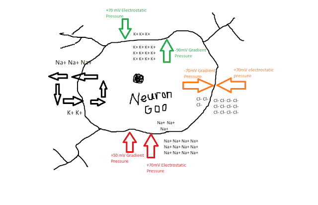
Ned the Neuron, filled with Neuron Goo. Note that the gradient and electrostatic pressures, expressed in microvolts (mV) have arbitrary signs; the point is to show that for an ion like chlorine, the pressures cancel out, while for an ion like potassium, there is slightly more pressure to exit the cell than enter it. Also, if you noticed that these values aren't 100% accurate, then congratu-frickin-lations, you're smarter than I am, but there is no way in HECK that I am redoing this in Microsoft Paint.


In addition to these passive forces, Hodgkin and Huxley also observed an active, energy-consuming force in maintaining the resting potential - a mechanism which exchanged potassium for sodium ions, by kicking out roughly three sodium ions for each potassium ion. Even with this pump though, there is still a whopping 120mV of pressure for sodium ions to enter. What prevents them from rushing in there and trashing the place?

Hodgkin and Huxley hypothesized that certain channels in the neuron membrane were selectively permeable, meaning that only specific ions could pass through them. Furthermore, channels could be either open or closed; for example, there may be sodium channels dotting the membrane, but at a resting potential they are usually closed. In addition, Hodgkin and Huxley thought that within these channels were gates that regulated whether the channel was open or closed, and that these gates could be in either permissive or non-permissive states. The probability of a gate being in either state was dependent on the voltage difference between the inside and the outside of the membrane.

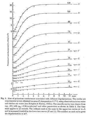
Although this all may seem conceptually straightforward, keep in mind that Hodgkin and Huxley were among the first to combine all of these properties into one unified model - something which could account for the conductances, voltage, and current, as well as how all of this affected the gates within each ion channel - and they were basically doing it from scratch. Also keep in mind that these crazy mofos didn't have stuff like Matlab or R to help them out; they did this the old-fashioned way, by changing one thing at a time and measuring that shit by hand. Insane. (Also think about how, in the good old days, people like Carthaginians and Romans and Greeks would march across entire continents for months, years sometimes, just to slaughter each other. Continents! These days, my idea of a taxing cardiovascular workout is operating a stapler.) To show how they did this for quantifying the relationship between voltage and conductance in potassium, for example, they simply applied a bunch of different currents, saw how it changed over time, and attempted to fit a mathematical function to it, which happens to fit quite nicely when you include n-gates and a fourth-power polynomial.


After a series of painstaking experiments and measurements, Hodgkin and Huxley calculated values for the conductances and equilibrium voltages for different ions. Quite a feat, when you couple that with the fact that they hunted down and killed their very own Giant Squid and then ripped a neuron out of its brain. Incredible. That is the very definition of alpha male behavior, and it's something I want all of my readers to emulate.
Table 3 from Hodgkin & Huxley (1952) showing empirical values for voltages and conductances, as well as the capacitance of the membrane.

The same procedure was used for the n, m, and h gates, which were also found to be functions of the membrane voltage. Once these were calculated, then the conductances and voltage potential could be found for any resting potential and any amount of injected current.

H & H's formulas for the n, m, and h gates as a function of voltage.

So where does that leave us? Since Hodgkin and Huxley have already done most of the heavy lifting for us, all we need to do is take their constants and equations they've already derived, and put it into a script that we can then run through Matlab. At some point, just to get some additional exercise, we may also operate a stapler.

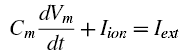
But stay focused here. Most of the formulas and constants can simply be transcribed from their papers into a Matlab script, but we also need to think about the final output that we want, and how we are going to plot it. Note that the original Hodgkin and Huxley paper uses a differential formula for voltage to tie together the capacitance and conductance of the membrance, e.g.:

We can use a method like Euler first-order approximation to plot the voltages, in which each time step is based off of the previous one which is added to a function multiplied by a time step; in the sample code below, the time step can be extremely small, thus giving a better approximation to the true shape of the voltage timecourse. (See the "calculate the derivatives" section below.)

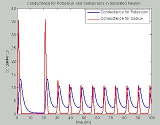
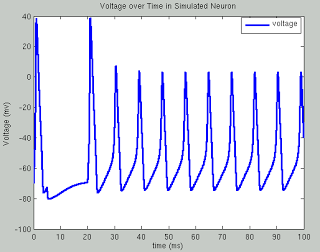
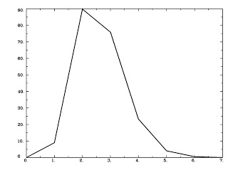
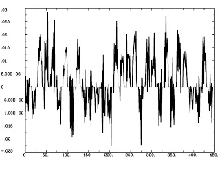
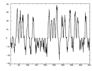
The following code runs a simulation of the Hodgkin Huxley model over 100 milliseconds with 50mA of current, although you are encouraged to try your own and see what happens. The sample plots below show the results of a typical simulation; namely, that the voltage depolarizes after receiving a large enough current and briefly becomes positive before returning to its previous resting potential. The conductances of sodium and potassium show that the sodium channels are quickly opened and quickly closed, while the potassium channels take relatively longer to open and longer to close.The point of the script is to show how equations from papers can be transcribed into code and then run to simulate what neural activity should look like under certain conditions. This can then be expanded into more complex areas such as memory, cognition, and learning.

The actual neuron, of course, is nowhere to be seen; and thank God for that, else we would run out of Giant Squids before you could say Jack Robinson.


Resources
Book of GENESIS, Chapter 4
Original Hodgkin & Huxley paper


%===simulation time===
simulationTime = 100; %in milliseconds
deltaT=.01;
t=0:deltaT:simulationTime;


%===specify the external current I===
changeTimes = [0]; %in milliseconds
currentLevels = [50]; %Change this to see effect of different currents on voltage (Suggested values: 3, 20, 50, 1000)

%Set externally applied current across time
%Here, first 500 timesteps are at current of 50, next 1500 timesteps at
%current of zero (resets resting potential of neuron), and the rest of
%timesteps are at constant current
I(1:500) = currentLevels; I(501:2000) = 0; I(2001:numel(t)) = currentLevels;
%Comment out the above line and uncomment the line below for constant current, and observe effects on voltage timecourse
%I(1:numel(t)) = currentLevels;


%===constant parameters===%
%All of these can be found in Table 3
gbar_K=36; gbar_Na=120; g_L=.3;
E_K = -12; E_Na=115; E_L=10.6;
C=1;


%===set the initial states===%
V=0; %Baseline voltage
alpha_n = .01 * ( (10-V) / (exp((10-V)/10)-1) ); %Equation 12
beta_n = .125*exp(-V/80); %Equation 13
alpha_m = .1*( (25-V) / (exp((25-V)/10)-1) ); %Equation 20
beta_m = 4*exp(-V/18); %Equation 21
alpha_h = .07*exp(-V/20); %Equation 23
beta_h = 1/(exp((30-V)/10)+1); %Equation 24

n(1) = alpha_n/(alpha_n+beta_n); %Equation 9
m(1) = alpha_m/(alpha_m+beta_m); %Equation 18
h(1) = alpha_h/(alpha_h+beta_h); %Equation 18


for i=1:numel(t)-1 %Compute coefficients, currents, and derivates at each time step
   
    %---calculate the coefficients---%
    %Equations here are same as above, just calculating at each time step
    alpha_n(i) = .01 * ( (10-V(i)) / (exp((10-V(i))/10)-1) );
    beta_n(i) = .125*exp(-V(i)/80);
    alpha_m(i) = .1*( (25-V(i)) / (exp((25-V(i))/10)-1) );
    beta_m(i) = 4*exp(-V(i)/18);
    alpha_h(i) = .07*exp(-V(i)/20);
    beta_h(i) = 1/(exp((30-V(i))/10)+1);
   
   
    %---calculate the currents---%
    I_Na = (m(i)^3) * gbar_Na * h(i) * (V(i)-E_Na); %Equations 3 and 14
    I_K = (n(i)^4) * gbar_K * (V(i)-E_K); %Equations 4 and 6
    I_L = g_L *(V(i)-E_L); %Equation 5
    I_ion = I(i) - I_K - I_Na - I_L;
   
   
    %---calculate the derivatives using Euler first order approximation---%
    V(i+1) = V(i) + deltaT*I_ion/C;
    n(i+1) = n(i) + deltaT*(alpha_n(i) *(1-n(i)) - beta_n(i) * n(i)); %Equation 7
    m(i+1) = m(i) + deltaT*(alpha_m(i) *(1-m(i)) - beta_m(i) * m(i)); %Equation 15
    h(i+1) = h(i) + deltaT*(alpha_h(i) *(1-h(i)) - beta_h(i) * h(i)); %Equation 16

end


V = V-70; %Set resting potential to -70mv

%===plot Voltage===%
plot(t,V,'LineWidth',3)
hold on
legend({'voltage'})
ylabel('Voltage (mv)')
xlabel('time (ms)')
title('Voltage over Time in Simulated Neuron')


%===plot Conductance===%
figure
p1 = plot(t,gbar_K*n.^4,'LineWidth',2);
hold on
p2 = plot(t,gbar_Na*(m.^3).*h,'r','LineWidth',2);
legend([p1, p2], 'Conductance for Potassium', 'Conductance for Sodium')
ylabel('Conductance')
xlabel('time (ms)')
title('Conductance for Potassium and Sodium Ions in Simulated Neuron')


What's in an SPM.mat File?

A while back I attempted to write up a document that summarized everything someone would need to know about using SPM. It was called, I believe, the SPM User's Ultimate Guide: For Alpha Males, By Alpha Males. The title was perhaps a little ambitious, since I stopped updating it after only a few dozen pages. In particular I remember a section where I attempted to tease apart everything contained within the SPM.mat files output after first- and second-level analyses. To me this was the most important section, since complex model setups could be executed fairly easily by someone with a good understanding of Matlab code, but I never completed it.

Fortunately, however, there is someone out there who already vivisected the SPM.mat file and publicly displayed its gruesome remains in the online piazza. Researcher Nikki Sullivan has written an excellent short summary of what each field means, broken down into neat, easily digestible categories. You can find it on her website here, and I have also copied and pasted the information below. It makes an excellent shorthand reference, especially if you've forgotten, for example, where contrast weights are stored in the structure, and don't want to go through the tedium of typing SPM, then SPM.xY, then SPM.xY.VY, and so on.

But if you've forgotten how to rock that body? Girl, ain't no remedy for that.


========================

details on experiment:


SPM.xY.RT - TR length (RT ="repeat time")
SPM.xY.P - matrix of file names
SPM.xY.VY - # of runs x 1 struct array of mapped image volumes (.img file info)
SPM.modality - the data you're using (PET, FMRI, EEG)
SPM.stats.[modality].UFp - critical F-threshold for selecting voxels over which the non-sphericity is estimated (if required) [default: 0.001]
SPM. stats.maxres - maximum number of residual images for smoothness estimation
SPM. stats.maxmem - maximum amount of data processed at a time (in bytes)
SPM.SPMid - version of SPM used
SPM.swd - directory for SPM.mat and img files. default is pwd

basis function:


SPM.xBF.name - name of basis function
SPM.xBF.length - length in seconds of basis
SPM.xBF.order - order of basis set
SPM.xBF.T - number of subdivisions of TR
SPM.xBF.T0 - first time bin (see slice timing)
SPM.xBF.UNITS - options: 'scans'|'secs' for onsets
SPM.xBF.Volterra - order of convolution
SPM.xBF.dt - length of time bin in seconds
SPM.xBF.bf - basis set matrix

Session Stucture:


user-specified covariates/regressors (e.g. motion)
SPM.Sess([sesssion]).C.C - [nxc double] regressor (c#covariates,n#sessions)
SPM.Sess([sesssion]).C.name - names of covariates
conditions & modulators specified - i.e. input structure array
SPM.Sess([sesssion]).U(condition).dt: - time bin length {seconds}
SPM.Sess([sesssion]).U(condition).name - names of conditions
SPM.Sess([sesssion]).U(condition).ons - onset for condition's trials
SPM.Sess([sesssion]).U(condition).dur - duration for condition's trials
SPM.Sess([sesssion]).U(condition).u - (t x j) inputs or stimulus function matrix
SPM.Sess([sesssion]).U(condition).pst - (1 x k) peri-stimulus times (seconds)
parameters/modulators specified
SPM.Sess([sesssion]).U(condition).P - parameter structure/matrix
SPM.Sess([sesssion]).U(condition).P.name - names of modulators/parameters
SPM.Sess([sesssion]).U(condition).P.h - polynomial order of modulating parameter (order of polynomial expansion where 0none)
SPM.Sess([sesssion]).U(condition).P.P - vector of modulating values
SPM.Sess([sesssion]).U(condition).P.P.i - sub-indices of U(i).u for plotting
scan indices for sessions
SPM.Sess([sesssion]).row
effect indices for sessions
SPM.Sess([sesssion]).col
F Contrast information for input-specific effects
SPM.Sess([sesssion]).Fc
SPM.Sess([sesssion]).Fc.i - F Contrast columns for input-specific effects
SPM.Sess([sesssion]).Fc.name - F Contrast names for input-specific effects
SPM.nscan([session]) - number of scans per session (or if e.g. a t-test, total number of con*.img files)

global variate/normalization details


SPM.xGX.iGXcalc - either "none" or "scaling." for fMRI usually is "none" (no global normalization). if global normalization is "Scaling", see spm_fmri_spm_ui for parameters that will then appear under SPM.xGX.

design matrix information:


SPM.xX.X - Design matrix (raw, not temporally smoothed)
SPM.xX.name - cellstr of parameter names corresponding to columns of design matrix
SPM.xX.I - nScan x 4 matrix of factor level indicators. first column is the replication number. other columns are the levels of each experimental factor. SPM.xX.iH - vector of H partition (indicator variables) indices
SPM.xX.iC - vector of C partition (covariates) indices
SPM.xX.iB - vector of B partition (block effects) indices
SPM.xX.iG - vector of G partition (nuisance variables) indices
SPM.xX.K - cell. low frequency confound: high-pass cutoff (secs)
SPM.xX.K.HParam - low frequency cutoff value
SPM.xX.K.X0 - cosines (high-pass filter)
SPM.xX.W - Optional whitening/weighting matrix used to give weighted least squares estimates (WLS).
  • if not specified spm_spm will set this to whiten the data and render the OLS estimates maximum likelihood i.e. W*W' inv(xVi.V).
SPM.xX.xKXs - space structure for K*W*X, the 'filtered and whitened' design matrix
SPM.xX.xKXs.X - Mtx - matrix of trials and betas (columns) in each trial
SPM.xX.xKXs.tol - tolerance
SPM.xX.xKXs.ds - vectors of singular values
SPM.xX.xKXs.u - u as in X u*diag(ds)*v'
SPM.xX.xKXs.v - v as in X u*diag(ds)*v'
SPM.xX.xKXs.rk - rank
SPM.xX.xKXs.oP - orthogonal projector on X
SPM.xX.xKXs.oPp - orthogonal projector on X'
SPM.xX.xKXs.ups - space in which this one is embedded
SPM.xX.xKXs.sus - subspace
SPM.xX.pKX - pseudoinverse of K*W*X, computed by spm_sp
SPM.xX.Bcov - xX.pKX*xX.V*xX.pKX - variance-covariance matrix of parameter estimates (when multiplied by the voxel-specific hyperparameter ResMS of the parameter estimates (ResSS/xX.trRV ResMS) )
SPM.xX.trRV - trace of R*V
SPM.xX.trRVRV - trace of RVRV
SPM.xX.erdf - effective residual degrees of freedom (trRV^2/trRVRV)
SPM.xX.nKX - design matrix (xX.xKXs.X) scaled for display (see spm_DesMtx('sca',... for details) SPM.xX.sF - cellstr of factor names (columns in SPM.xX.I, i think) SPM.xX.D - struct, design definition SPM.xX.xVi - correlation constraints (see non-sphericity below) SPM.xC - struct. array of covariate info

header info


SPM.P - a matrix of filenames
SPM.V - a vector of structures containing image volume information.
SPM.V.fname - the filename of the image.
SPM.V.dim - the x, y and z dimensions of the volume
SPM.V.dt - A 1x2 array. First element is datatype (see spm_type). The second is 1 or 0 depending on the endian-ness.
SPM.V.mat- a 4x4 affine transformation matrix mapping from voxel coordinates to real world coordinates.
SPM.V.pinfo - plane info for each plane of the volume.
SPM.V.pinfo(1,:) - scale for each plane
SPM.V.pinfo(2,:) - offset for each plane The true voxel intensities of the jth image are given by: val*V.pinfo(1,j) + V.pinfo(2,j)
SPM.V.pinfo(3,:) - offset into image (in bytes).If the size of pinfo is 3x1, then the volume is assumed to be contiguous and each plane has the same scalefactor and offset.

structure describing intrinsic temporal non-sphericity


SPM.xVi.I - typically the same as SPM.xX.I SPM.xVi.h - hyperparameters
SPM.xVi.V xVi.h(1)*xVi.Vi{1} + ...
SPM.xVi.Cy - spatially whitened (used by ReML to estimate h)
SPM.xVi.CY - <(Y - )*(Y - )'>(used by spm_spm_Bayes)
SPM.xVi.Vi - array of non-sphericity components

  • defaults to {speye(size(xX.X,1))} - i.ii.d.
  • specifying a cell array of contraints ((Qi)
  • These contraints invoke spm_reml to estimate hyperparameters assuming V is constant over voxels that provide a high precise estimate of xX.V
SPM.xVi.form - form of non-sphericity (either 'none' or 'AR(1)')
SPM.xX.V - Optional non-sphericity matrix. CCov(e)sigma^2*V.
  • If not specified spm_spm will compute this using a 1st pass to identify signifcant voxels over which to estimate V. A 2nd pass is then used to re-estimate the parameters with WLS and save the ML estimates (unless xX.W is already specified)
 

filtering information


SPM.K - filter matrix or filtered structure:
  • SPM.K(s) - struct array containing partition-specific specifications
  • SPM.K(s).RT - observation interval in seconds
  • SPM.K(s).row - row of Y constituting block/partitions
  • SPM.K(s).HParam - cut-off period in seconds
  • SPM.K(s).X0 - low frequencies to be removed (DCT)
  • SPM.Y - filtered data matrix
 

masking information


SPM.xM - Structure containing masking information, or a simple column vector of thresholds corresponding to the images in VY.
SPM.xM.T - [n x 1 double] - Masking index
SPM.xM.TH - nVar x nScan matrix of analysis thresholds, one per image
SPM.xM.I - Implicit masking (0 --> none; 1 --> implicit zero/NaN mask)
SPM.xM.VM - struct array of mapped explicit mask image volumes
SPM.xM.xs - [1x1 struct] cellstr description

design information (self-explanatory names, for once) 


SPM.xsDes.Basis_functions - type of basis function
SPM.xsDes.Number_of_sessions
SPM.xsDes.Trials_per_session
SPM.xsDes.Interscan_interval
SPM.xsDes.High_pass_Filter
SPM.xsDes.Global_calculation
SPM.xsDes.Grand_mean_scaling
SPM.xsDes.Global_normalisation

details on scannerdata (e.g. smoothness) 


SPM.xVol - structure containing details of volume analyzed
SPM.xVol.M- 4x4 voxel --> mm transformation matrix
SPM.xVol.iM - 4x4 mm --> voxel transformation matrix
SPM.xVol.DIM - image dimensions - column vector (in voxels)
SPM.xVol.XYZ - 3 x S vector of in-mask voxel coordinates
SPM.xVol.S- Lebesgue measure or volume (in voxels)
SPM.xVol.R- vector of resel counts (in resels)
SPM.xVol.FWHM - Smoothness of components - FWHM, (in voxels)

info on beta files:


SPM.Vbeta - struct array of beta image handles
SPM.Vbeta.fname - beta img file names
SPM.Vbeta.descrip - names for each beta file

info on variance of the error


SPM.VResMS - file struct of ResMS image handle
SPM.VResMS.fname - variance of error file name

info on mask


SPM.VM - file struct of Mask image handle
SPM.VM.fname - name of mask img file

contrast details (added after running contrasts)


SPM.xCon - Contrast definitions structure array
  • (see also spm_FcUtil.m for structure, rules &handling)
SPM.xCon.name - Contrast name
SPM.xCon.STAT - Statistic indicator character ('T', 'F' or 'P')
SPM.xCon.c - Contrast weights (column vector contrasts)
SPM.xCon.X0 - Reduced design matrix data (spans design space under Ho)
  • Stored as coordinates in the orthogonal basis of xX.X from spm_sp
  • (Matrix in SPM99b)
  • Extract using X0 spm_FcUtil('X0',...
SPM.xCon.iX0 - Indicates how contrast was specified:
  • If by columns for reduced design matrix then iX0 contains the column indices.
  • Otherwise, it's a string containing the spm_FcUtil 'Set' action: Usually one of {'c','c+','X0'} defines the indices of the columns that will not be tested. Can be empty.
SPM.xCon.X1o - Remaining design space data (X1o is orthogonal to X0)
  • Stored as coordinates in the orthogonal basis of xX.X from spm_sp (Matrix in SPM99b) Extract using X1o spm_FcUtil('X1o',...
SPM.xCon.eidf - Effective interest degrees of freedom (numerator df)
  • Or effect-size threshold for Posterior probability
SPM.xCon.Vcon - Name of contrast (for 'T's) or ESS (for 'F's) image
SPM.xCon.Vspm - Name of SPM image

Multi-Variate Pattern Analysis (MVPA): An Introduction

Alert reader and fellow brain enthusiast Keith Bartley loves MVPA, and he's not ashamed to admit it. In fact, he loves MVPA so much that he was willing to share what he knows with all of us, as well as a couple of MVPA libraries he has ported from Matlab to Octave.

Why don't I write a post on MVPA, you ask? Maybe because I don't know doodley-squat about it, and maybe because I'm man enough to admit what I don't know. In my salad days when I was green in judgment I used to believe that I needed to know everything; nowadays, I get people to do that for me. This leaves me more time for gentlemanly activities, such as hunting, riding, shooting, fishing, and wenching.

So without further delay, here it is: An introduction to MVPA for those who are curious about it and maybe even want to do it themselves, but aren't exactly sure where to start. Be sure to check out the links at the end of the post for links to Keith's work, as well as Octave distributions he has been working on.


==================================

Well, it had to happen sometime. Time to call out the posers. Those who would bend neuroscience to their evil will. Where to start? How about the New York Times. Oh, New York Times. You've managed to play both sides of this coin equally well. Creating a neuroimaging fallout with bad reports, then throwing out neuroscience studies altogether ("The brain is not the mind" <- What? Stop. Wait, who are you again? Just stop). What's to be said for those few that rise above the absolutes of "newspaper neuroscience", and simply report findings, not headline grabbing inferences? Should we be opposed to gained knowledge, or seek to better understand the details? Boring you say? Pfft. Then you have yet to know the neuroscience I know.

As an example, a recent NYT article suggested that activation in both the primary auditory and visual cortices in response to an iPhone ring alone demonstrated that people were seeing the iPhone in their mind's eye.

...
This is a completely RIDICULOUS notion to suggest from univariate GLM BOLD response alone. But can we ever really know what a person sees in their mind's eye or hears in their mind's ear? Remember, good science happens in the setup, not the interpretation.

You may have heard of an increasingly implemented form of machine classification in brain-imaging dubbed Multi-Variate Pattern Analysis (MVPA). If you prefer the term "mind reading", sure go ahead, but remember to bring your scientific floaties, lest you drown from the lack of understanding as it escapes the proverbial lungs of your deoxygenated mind. Before you know it, you'll be believing things like this:


Verbose laughter ensues. Close, but no Vicodin. How does MVPA of BOLD responses really work?


Source: Kaplan & Meyer, 2011

By first training a program to recognize a pattern, in much the same way you might visually recognize a pattern, we can quantitatively measure the similarity or dissimilarity of patterns in response to differing conditions. But what does this have to do with knowing what a person might see in their mind? I recently compiled some soundless videos for a demonstration of just this. Watch them fullscreen for the greatest effect.


It's likely that the sound of coins clanking, a car crashing, or Captain Kirk screaming "KAHHHHN!!!" registered in your mind, and thus created distinct neural representations in your primary auditory cortex. If we train a machine classifier to recognize your brain's patterned neural response to the sound, we can then ask the classifier to guess which among all these stimuli your brain is distinctly representing in the absence of sound. If the machine classifier is successful statistically more than null permutations of chance, THEN we can MAYBE begin to suggest a top-down neural mechanism of alternate sensory modality stimulation. 

BUT, I promised you details, and details you shall have!

As a fan of Princeton's MVPA Matlab toolbox, opening it up for people without access to a Matlab license seemed like the next most logical step, prompting me to convert the toolbox, as well as its implementations of SPM and AFNI-for-MATLAB, to one unitary Octave distribution. Below is a link to my website and Github page. There you will find setup instructions as well as tutorial data and a script that Dr. Marc Coutanche (See his rigorously awesome research in MVPA here) and I implemented in a recent workshop. Coded are step-by-step instructions to complete what is a research caliber implementation of pattern analysis. Learn it, live it, repeat it, and finally bask in your ability to understand something that would make your grandma's head explode (See the Flynn Effect for possible explanation there). As with anything I post, if you have questions, comments, or criticisms, feel free to message me through any medium of communication ...unless you are a psychic. I'd like to keep my mind's ear to myself. 


De Profundis

Since school started back up a little over a month ago, I've been teaching my own introductory psychology course - the first one I've ever taught. It's been great; when I do it, I feel happy, energized, useful. Not only do I get to teach a couple of hundred persons, some of whom really like the class, but I even get to write my own test questions. If ten years ago you told me I would be lecturing in front of college students and creating exams, I would've told you to go kick rocks. But oddly enough, I enjoy it. For instance, I get to come up with test questions like this:

Sigmund Freud was:

A) correct
B) completely insane
C) a cocaine abuser
D) all of the above


Understandably, the writing here took a hit, as I left the mistress of my youth, blogging, for the wife of mine age, teaching. I figured that whatever basics someone needed to know they could find somewhere in the archives. I thought that I probably was spending too much time on it anyway, feeling a distinct negative correlation between the amount of material that was posted on here and my actual productivity as a researcher. Maybe once in while, I thought, I would post about relationship advice, or books I was reading, or possibly a sequel to my post about erotic neuroimaging journal titles. In any case, though, I thought that I written most of what I had wanted to. Quod scripsi, scripsi.

However, I got a jolt a couple of days ago when the government shut down. Normally this wouldn't affect me all that much, except for the AFNI developers sending out a warning that the entire website would be shut down and the message boards closed until further notice. Apparently it's illegal for federal employees to use government emails for correspondence during a shutdown. No more AFNI support; no more new AFNI materials; no more infamous Bob Cox insults, put-downs, and slams. All gone.

Which made me realize, God forbid, that AFNI won't be around forever. I doubt that even fMRI will be all that popular twenty, thirty years from now, as technology progresses and we find some new way to image the brain yet still get significant results no matter how badly we screw up. But the need for understanding the processes will still be there; people will always want easy, accessible introductions for learning new tools and new methods. So I will continue to do that, no matter how incomplete my understanding, no matter how many miles I run, no matter how many jars of Nutella I devour. And that's a campaign promise.

At least one researcher out there has offered to write about topics that I am either entirely ignorant of, or only have a limited grasp. Starting soon, I will begin to interleave some of those posts with what I write to make the blog more centralized for information relating to fMRI. In the meantime, if anyone reading wants to contribute, just let me know. We'll see how it works out.


Real Ultimate Power

I once read an article by a man who guaranteed that by following a series of simple steps, your blog would become famous overnight and make you filthy rich. He pointed to himself as a case study, having founded a blog devoted to nutrition advice and dietary tips for Caucasian males. He called it White Man's Secret. Within weeks, he claimed, he had millions of unique hits every single day from all over the world. Tens of thousands of women left their husbands or lovers and became his willing slaves. He was elected president of his Rotary chapter and was voted Best Table Topics Speaker at his local Toastmasters five times in a row. And he had done it all by following a series of simple steps that anybody could do.

Most important, he said - or screamed, rather, since everything was in upper case capital letters - was to never apologize for failing to update regularly. People wouldn't even notice it, he said, unless you called attention to it. He recommended treating readers like any one of the members of his now-overflowing seraglio - by playing with their emotions through deliberate neglect. Then, when they were at their most desperate, you would give them some attention. Not much. Just enough for them to become dependent on you.

This, he said, was an expression of power. Real Ultimate Power.

________________________________________


My reason for neglect isn't nearly as insidious. It's because I've been running too much.

A few weeks ago when I visited home I sat down with my dad and a calendar and we made a training program leading up to the Indianapolis marathon in November. At the beginning of each week he wrote the number of weeks left until race day. So, "12," "11," "10," and so on, until "0." Then in each cell of the calendar we calculated how many workouts and how many miles I would need to run to fill a weekly quota. We determined this using Jack Daniels' Running Formula.

I'm not talking about the stuff created by yeast poop. Jack Daniels is a real person. He is a coach with a doctorate in exercise physiology and fifteen years ago he published a book called Daniels' Running Formula. He also popularized the use of a physiological measurement called VDOT, which measures the maximum amount of oxygen used by the body. I have had my VDOT measured a couple of times by exercise physiologists, and both times the process was extremely uncomfortable. They put you on a treadmill and stick a tube in your mouth and then pinch your nostrils closed with a clothespin. You then start running, and the treadmill speed and incline increases every minute or so until you can't run anymore.

The last time I did this, the researchers told me that my VDOT was seventy-point-three. Jack Daniels has a specific workout plan for nearly any VDOT number. And so seventy-point-three was the number my dad and I were using when we filled out the calendar.

________________________________________


Here is what Jack Daniels says I should do in a typical week:

Sunday: 13-15 miles at marathon pace (5:40/mile); 2 miles warmup, 2 miles cooldown.
Monday: 10 miles
Tuesday: 12 miles in the morning, 4 miles in the evening
Wednesday: 8 mile recovery run
Thursday: 2 mile warmup. 2x12 minutes of anaerobic threshold pace (5:20/mile). 4 mile recovery jog followed by another 12 minutes anaerobic threshold pace (5:20/mile).
Friday: 12 miles
Saturday: 12 miles in the morning, 6 miles in the evening


When I read this I thought that Jack Daniels was nuttier than squirrel shit. Obviously there are some people who disagree; there are some out there who think this is easy and no big deal. Fly them.

I've stuck with it nonetheless; and the odd thing is, it seems to be working. My runs are getting easier; workouts are getting better; I feel more prepared and more motivated. The only problem is that during the day I'm too tired to do anything else. I get up in the morning around six and am usually done around seven-thirty. For the next hour or so I stretch a little bit and drink chocolate soy milk straight out of the carton. I put a towel on the living room floor and lie there sweating, and sometimes put on music I checked out from the library. For the past month or so I've been listening primarily to jazz - Duke Ellington, Earl Klugh, Ella Fitzgerald, Bill Evans, Thelonious Monk, to name a few. I listen to some classical stuff as well. This morning as I laid on my sweat-soaked towel on the floor, I listened to a sonata by Ravel. It was heavenly.

Then I go to work and feel the slow burn in my legs for the rest of the day. In a way it feels almost pleasurable. And then when I get home sometimes I run again. Sometimes I will see other people out there running, and wonder about whether they are faster than I am.

Some would call this insecurity. They're probably right. In any case, I like to call it competitiveness.

________________________________________


Speaking of competitiveness: A couple of years ago a girl told me that one of her previous boyfriends had run a marathon in two hours and thirty-two minutes. At the time, that was faster than I had run a marathon, and so naturally I became insanely jealous. It didn't help that I was hopelessly in love with this girl. The fact that she had dated someone with a faster marathon time was an insult to me.

For the next nine months I trained like a banshee and that summer I ran a marathon in two hours and thirty minutes. Somewhere in the back of my mind I was convinced that when I told her my marathon time, she would rip off all her clothes with uncontrollable passion.

That never happened. The next time she saw me she didn't even take off her sunglasses. Things have been pretty much the same.

________________________________________

By the way: When someone wants to run with you, wait for a really cold morning and tell them that you want to run then. At the last minute they will come up with an excuse not to go.

You know why? Because running in the cold sucks.


Pro Tip: Changing SPM Output Files


A couple of weeks ago, alert reader Paula DiNoto asked about how to output SPM files in NIFTI format instead of ANALYZE (.hdr/.img). Apparently, for those of you bleeding-edge adrenaline junkies who just have to have the latest thing, SPM12 doesn't give you this option in the interface. SPM5, however - you know, the one that the rest of us barbarians use - still does. (I'll save my gloating for when I meet you face-to-face at the conferences.)

Getting back to the story, I had to admit to Paula that I was, for the first time in my life, unable to figure out how to troubleshoot the problem. However, this was merely a ruse to get Paula motivated; she ended up solving the problem by changing "spm_defaults.m" and changing the default.images.format field to 'nii'. Obviously I already knew this, but I was pleased to see her figure it out for herself.


Thanks again to Paula, whom I once called, in a moment of self-forgetfulness, the most wonderful person I had ever met.

Back Next Week


Fellow brainbloggers,

I'll be going home for a few days - running a few races, seeing a few friends, eating a few pizzas, kicking back a few Shirley Temples. Getting that messed up on Sprite and grenadine means that updates may be scarce. When I return, though, I will be going to FMRI pound-town on those resting-state analyses and hit you with the full report as promised.


Eric my man, take us outta here.

Psychophysiological Interactions Explained

That last tutorial on psychophysiological interactions - all thirteen minutes of it - may have been a little too much to digest in one sitting. However, you also don't understand what it's like to be in the zone, with the AFNI commands darting from my fingertips and the FMRI information tumbling uncontrollably from my lips; sometimes I get so excited that I accidentally spit a little when I talk, mispronounce words like "particularly," and am unable to string two coherent thoughts together. It's what my dating coach calls the vibe.

With that in mind, I'd like to provide some more supporting commentary. Think of it as supplementary material - that everybody reads!

Psychophysiological interactions (PPIs) are correlations that change depending on a given condition, just as in statistics. (The concept is identical, actually.) For example: Will a drug affect your nervous system differently from a placebo depending on whether you have been drinking or not? Does the effectiveness of Old Spice Nocturnal Creatures Scent compared to Dr. Will Brown's Nutty Time Special Attar (tm) depend on whether your haberdasher is Saks Fifth Avenue, or flophouse? Does the transcendental experience of devouring jar after jar of Nutella depend on whether you are alone, or noshing on it with friends? (Answer: As long as there's enough to go around, let the good times roll, baby!)

So much for the interaction part, but what about this psychophysiological thing? The "psychophysiological" term is composed of two parts, namely - and I'm not trying to insult your intelligence here - a psychological component and a physiological component. The "psychological" part of a PPI refers to which condition your participant was exposed to; perhaps the condition where she was instructed to imagine a warm, fun, exciting environment, such as reading Andy's Brain Blog with all of her sorority sisters during a pajama party on a Saturday night and trying to figure out what, exactly, makes that guy tick. Every time she imagines this, we code it with a 1; every time she imagines a contrasting condition, such as reading some other blog, we code that with a -1. And everything else gets coded as a 0.

Here are pictures to make this more concrete:

Figure 1: Sorority girls reading Andy's Brain Blog (aka Condition 1)
Figure 2: AvsBcoding with 1's, -1's, and 0's
The physiological component, on the other hand, simply refers to the underlying neural activity. Remember, however, that what we see in a typical FMRI timeseries isn't the actual neural activity; it's neural activity that has been smeared (i.e., convolved) with the hemodynamic response function, or HRF. To convert this back to the neural timeseries, we de-smear (i.e., deconvolve) the timeseries by removing the HRF - similar to a Fourier analysis if you have done one of those. (You have? NERD!)

To summarize: we assume that the observed timeseries is a convolution of the underlying neural activity with the HRF. Using NA for neural activity, HRF for the gamma response function, and (x) for the Kroenecker product, symbolically this looks like:

TimeSeries = NA (x) HRF

To isolate the NA part of the equation, we extract the TimeSeries from a contrast or some anatomically defined region, either using the AFNI Clusterize GUI and selecting the concatenated functional runs as an Auxiliary TimeSeries, or through a command such as 3dmaskave or 3dmaskdump. (In either case, make sure that the text file is one column, not one row; if it is one row, use 1dtranspose to fix it.) Let's call this ideal time series Seed_ts.1D.

Next, we generate an HRF using the waver command and shuffle it into a text file:

waver -dt [TR] -GAM -inline 1@1 > GammaHR.1D

Check this step using 1dplot:

1dplot GammaHR.1D

And you should see something like this:

Now that we have both our TimeSeries and our HRF, we can calculate NA, the underlying neural activity, using 3dTfitter (the -Faltung option, by the way, is German for "deconvolution"):

3dTfitter -RHS Seed_ts.1D -FALTUNG GammaHR.1D Seed_Neur 012 0

This will tease apart GammaHR.1, from the TimeSeries Seed_ts.1D, and store it in a file called Seed_Neur.1D. This should look similar to the ideal time course we generated in the first step, except now it is in "Neural time":

1dplot Seed_Neur.1D


Ausgezeichnet! All we have to do now is multiply this by the AvsBcoding we made before, and we will have our psychophysiological interaction!

1deval -a Seed_Neur.1D -b AvsBcoding.1D -expr 'a*b' -prefix Inter_neu.1D

This will generate a file, Inter_neu.1D, that is our interaction at the neural level:

1dplot Inter_neu.1D

And, finally, we take it back into "BOLD time" by convolving this timeseries with the canonical HRF:

waver -dt 2 -GAM -input Inter_neu.1D -numout [numTRs] > Inter_ts.1D

1dplot Inter_ts.1D

Let's pause and review what we've done so far:
  1. First, we extracted a timeseries from a voxel or group of voxels somewhere in the brain, either defined by a contrast or an anatomical region (there are several other ways to do this, of course; these are just the two most popular);
  2. We then created a list of 1's, -1's, and 0's for our condition, contrasting condition, and all the other stuff, with one number for each TR;
  3. Next, we created a Gamma basis function using the waver command, simulating the canonical HRF;
  4. We used 3dTfitter to decouple the HRF from the timeseries, moving from "BOLD time" to "Neural time";
  5. We created our psychophysiological interaction by multiplying our AvsBcoding by the Neural TimeSeries; and
  6. Convolved this interaction with the HRF in order to move back to "BOLD time".

Our last step is to enter this interaction and the region's timeseries into our model. Since we are entering this into the model directly as is, and since we are not convolving it with anything, we will use the -stim_file option. Also remember to not use the -stim_base option, which is usually paired with -stim_file; we are still estimating parameters for this regressor, not just including it in the baseline model.

Below, I have slightly modified the 3dDeconvolve script used in the AFNI_data6 directory. The only two lines that have been changed are the stim_file options for regressors 9 and 10:

 #!/bin/tcsh

set subj = "FT"

# run the regression analysis
3dDeconvolve -input pb04.$subj.r*.scale+orig.HEAD                       \
    -polort 3                                                           \
    -num_stimts 10                                                       \
    -stim_times 1 stimuli/AV1_vis.txt 'BLOCK(20,1)'                     \
    -stim_label 1 Vrel                                                  \
    -stim_times 2 stimuli/AV2_aud.txt 'BLOCK(20,1)'                     \
    -stim_label 2 Arel                                                  \
    -stim_file 3 motion_demean.1D'[0]' -stim_base 3 -stim_label 3 roll  \
    -stim_file 4 motion_demean.1D'[1]' -stim_base 4 -stim_label 4 pitch \
    -stim_file 5 motion_demean.1D'[2]' -stim_base 5 -stim_label 5 yaw   \
    -stim_file 6 motion_demean.1D'[3]' -stim_base 6 -stim_label 6 dS    \
    -stim_file 7 motion_demean.1D'[4]' -stim_base 7 -stim_label 7 dL    \
    -stim_file 8 motion_demean.1D'[5]' -stim_base 8 -stim_label 8 dP    \
    -stim_file 9 Seed_ts.1D -stim_label 9 Seed_ts    \
    -stim_file 10 Inter_ts.1D -stim_label 10 Inter_ts    \

    -gltsym 'SYM: Vrel -Arel' -x1D X.xmat.1D -tout -xjpeg X.jpg                             \
    -bucket stats_Inter.$subj -rout


This will generate a beta weights for the Interaction term, which can then be taken to a group-level analysis using your command of choice. You can also do this with the R-values, but be aware that 3dDeconvolve will generate R-squared values; you will need to take the square root of these and then apply a Fisher's R-to-Z transform before you do a group analysis. Because of the extra steps involved, and because interpreting beta coefficients is much more straightforward, I recommend sticking with the beta weights.

Unless you're a real man like my dating coach, who recommends alpha weights.

Context-Dependent Correlations (aka PsychoPhysiological Interactions)

As promised, here is the tutorial on context-dependent correlations. Just to confuse you a little, I also refer to them as psychophysiological interactions, or PPIs, because different people call it different things. Kind of like how some people call me Andy, but other people call me Andy Pandy. Specifically, my mom.


More details about PPIs - and my childhood - coming up soon, but first I have a level 2 scanning emergency to take care of tonight. And I mean that in all seriousness, not the way I usually toss that phrase around - to get out of awkward dates. And now you know, ladies!

Future Functional Connectivity Tutorials, and Other Updates

A few notes:

1) The previous functional connectivity posts and tutorials are cribbed from Gang Chen's homepage, which is available here. Kind of like the way I crib quotations and passages from authors that no one reads anymore, and then pass it off as my own style to boost my pathologically low self-esteem. Keep in mind that most of these demonstrations deal with a single subject and simplified situations that you probably will not encounter in your research. Given these contrived examples, most of the results generated in these demos are relatively meaningless; it's up to you to learn and understand the concepts, and then apply them to your own data and make your own inferences. My task which I am trying to achieve is, by the power of Youtube tutorials, to make you hear, to make you feel — it is, before all, to make you understand. That — and no more, and it is everything. (That was Conrad, by the way.)

2) A lot of you - I'm talking a LOT of you players - have been making requests for MELODIC tutorials and resting state analyses in FSL. All I can say is, we'll get there, in time. Before that, however, I believe AFNI is better suited for building up one's intuition, and so we will be working through a few more connectivity topics in AFNI - specifically, context-dependent correlations, beta series correlations, and resting state connectivity. After that we will again cover the same concepts, but applied in FSL - by which time, given my glacial pace, either FMRI will have become a passé technique or the Andromeda galaxy will have crashed into us.

3) Recently you may have noticed the "Donate" button on the right sidebar of the blog. This was done at the request of one reader who felt the powerful, irrational urge to loosen his purse-strings and give some alms out of the goodness of his heart, which is located somewhere way, way down there, somewhere nearabouts the cockles. Although I can't fully understand this behavior - even less than I can understand why there is someone who still has purse-strings, or what cockles are, exactly - nevertheless it helps satisfy my cupidity and strokes my ego. Furthermore, in addition to serving Mammon, these tokens of gratitude motivate me to regularly produce new material and, as a bonus, help me to continue procrastinating on my dissertation. Now that's what I call a win-win-win.

4) Also, at least one of you has mailed me a two-pack of Nutella. This has pleased me greatly. My brain needs hazelnut spread for fuel, and the more it has, the hotter and better it burns.

5) If everything goes according to plan, we should cover context-dependent correlations this weekend, beta series correlations next week, and resting-state connectivity the week after that.

Lunch in Paris, dinner in London, comrade.