Neuroanatomy Made Fun

For those of you currently studying neuroanatomy, or for those who are just curious, Youtube user hyperhighs has posted an incredibly detailed set of drawings of the major components of the brain and nervous system. These gorgeous renderings teach you several important things about the brain, such as where it is and what it looks like. His channel also includes drawings and tutorials of cell physiology, cardiovascular function, and lipoprotein physiology, to name a few.

This guy helped me out a lot in my studying, and I hope it is of use to you as well. He also has this super chill music going on in the background all the time, which I want.

FSL Tutorial 2: FEAT (Part 3): For The Wind

Pictured: FSL User

[Before we begin: According to my traffic sources, the majority of my viewers, outside of the United States, are from Russia. If the history books I have read and the video games I have played are any guide, they are probably visiting this site in order to learn enough about cognitive neuroscience to produce some kind of supersoldier in order to restore communist hardliners to power and launch an assault on America. So, to all of my Russian readers: Hola!]

Finally, we have arrived at the end of the FEAT interface. The last two tabs, post-stats and registration, allow the user to specify how the results will be visualized, what kinds of multiple comparison corrections to carry out, and how to register and normalize the data.

One might wonder why FSL chooses to perform coregistration and normalization as the last step, instead of at a previous step in the preprocessing pipeline as do other software analysis packages. The reasoning is that because these steps introduce spatial correlations, it is better to introduce them after having run the statistical analysis, in order to prevent any sort of biases that may be introduced into the data as a result of applying these steps. Personally, I don't think it matters that much either way, since you have to do it at some point; however, that is the way it is built into the FSL stream, and if you don't like it, tough bananas.

Most of the defaults are fine; the only tab that requires any input before you can move forward is the Registration tab, which requires a skullstripped brain to normalize to a standardized space. This includes atlases such as Talairach or Montreal Neurological Institute (MNI), although I believe FSL only uses MNI. The point of normalization is that every subject's brain will be twisted, rotated, warped, and undergo various other uncomfortable transformations until it is located within a box that has equal dimensions to the standard space. Furthermore, certain anatomical landmarks will be at a specific coordinate position relative to every other part of the brain; for example, in Talairach space, the anterior commissure - a bundle of nerve fibers connecting the hemispheres, located at the base of the anterior columns of the fornix - will be positioned at coordinates 0, 0, 0. Thus, according to the Talairach atlas in this example, any other brain regions can be defined based on their distance from this origin (although the researcher should always check to make sure that what the atlas says matches up with what is directly in front of him).

A couple of other useful options are in the post-stats tab. For example, Pre-threshold masking allows the user to perform region of interest (ROI) analyses which define an a priori region either based on anatomical regions defined by an atlas or a binary mask generated by a program like Marsbar. Contrast masking has a similar role, masking out certain regions of the brain based on whether they are covered by another contrast in the analysis; although caution should be exercised here as well, in order to make sure that the masking contrast is orthogonal to the one being investigated. For more information about ROI analyses, as well as potential pitfalls, see an earlier post about the topic.

More tutorials will be up soon to guide the user through what all those HTML output files mean, as well as looking at and interpreting results.

Bayesian Approaches to fMRI: Thoughts

Pictured: Reverend Thomas Bayes, Creator of Bayes' Theorem and Nerd Baller

This summer I have been diligently writing up my qualification exam questions, which will effect my entry into dissertation writing. As part of the qualification exam process I opted to perform a literature review on Bayesian approaches to fMRI, with a focus on spatial priors and parameter estimation at the voxel level. This necessarily included a thorough review of the background of Bayesian inference, over the course of which I gradually became converted to the view that Bayesian inference was, indeed, more useful and more sophisticated than traditional null hypothesis significance testing (NHST) techniques, and that therefore every serious scientist should adopt it as his statistical standard.

At first, I tended to regard practitioners of Bayesian inference as seeming oddities, harmless lunatics so convinced of the superiority of their technique as to come across as almost condescending. Like all good proselytizers, Bayesian practitioners appear to be appalled by the putrid sea of misguided statistical inference in which their entire field had foundered, regarding their benighted colleagues as doomed unless they were injected with the appropriate Bayesian vaccine. And in no place was this zeal more evident than their continual attempts to sap the underlying foundations of NHST and the assumptions on which it rested. At the time I considered these differences between the two approaches to be trivial, mostly because I convinced myself that any overwhelmingly large effect size acquired in NHST would be essentially equivalent to a parameter estimate calculated by the Bayesian approach.

Bayesian Superciliousness Expressed through Ironic T-shirt

However, the more I wrote, the more I thought to myself that proponents of Bayesian methods may be on to something. It finally began to dawn on me that rejecting the null hypothesis in favor of an alternative hypothesis, and actually being able to say something substantive about the alternative hypothesis itself and compare it with a range of other models, are two very different things. Consider the researcher attempting to make the case that shining light in someone's eyes produces activation in the visual cortex. (Also consider the fact that doing such a study in the good old days would get you a paper into Science, and despair.) The null hypothesis is that shining light into someone's eyes should produce no activation. The experiment is carried out, and a significant 1.0% signal change is observed in the visual cortex, with a confidence interval from [0.95, 1.05]. The null hypothesis is rejected and you accept the alternative hypothesis that shining light in someone's eyes elicits greater neural activity in this area than do periods of utter and complete darkness. So far, so good.

Then, suddenly, one of these harmless Bayesian lunatics pops out of the bushes and points out that, although a parameter value has been estimated and a confidence interval calculated stating what range of values would not be rejected by a two-tailed significance test, little has been said about the credibility of your parameter estimate. Furthermore, nothing has been said at all about the credibility of the alternative hypothesis, and how much more believable it should be as compared to the null hypothesis. These words shock you so deeply that you accidentally knock over a nearby jar of Nutella, creating a delicious mess all over your desk and reminding you that you really should screw the cap back on when you are done eating.

Bayesian inference allows the researcher to do all of the above mentioned in the previous paragraph, and more. First, it has the advantage of being uninfluenced by the intentions of the experimenter, the knowledge of which is inherently murky and unclear, but on which NHST "critical" values are based. (More on this aspect of Bayesian inference, as compared to NHST, can be found in a much more detailed post here.) Moreover, Bayesian analysis sheds light on concepts common to both Bayesian and NHST approaches while pointing out the disadvantages of the latter and outlining how these deficiencies are addressed and mitigated in the former, whereas the converse approach is not true; this stems from the fact that Bayesian inference is more mathematically and conceptually coherent, providing a single posterior distribution for each parameter and model estimate without falling back on faulty, overly conservative multiple correction mechanisms which punish scientific curiosity. Lastly, Bayesian inference is more intuitive. We should intuitively expect our prior beliefs to influence our interpretation of posterior estimates, as more extraordinary claims should require correspondingly extraordinary evidence.

Having listened to this rhapsody on the virtues and advantages of going Bayesian, the reader may wonder how many Bayesian tests I have ever performed on my own neuroimaging data. The answer is: None.

Why is this? First of all, considering the fact that a typical fMRI dataset is comprised of hundreds of thousands of voxels, and given current computational capacity, Bayesian inference for an single neuroimaging session can take prohibitively long amounts of time. Furthermore, the only fMRI analysis package I know of that allows for Markov-Chain Monte Carlo (MCMC) sampling at each voxel is FSL's FLAME 1+2, although this procedure can take on the order of days for a single subject, and the results usually tend to be more or less equal to what would be produced through traditional methods. Add on top of this models which combine several levels of priors and hyperparameters which mutually constrain each other, and the computational cost increases even more exponentially. One neuroimaging technique which uses Bayesian inference in the form of spatial priors in order to anatomically constrain the strength and direction of connectivity - an approach known as dynamic causal modeling (DCM; Friston et al, 2003) - is relatively unused among the neuroimaging community, given the complexity of the approach (at least, outside of Friston's group). Because of these reasons, Bayesian inference has not gained much traction in the neuroimaging literature.

However, some statistical packages do allow for the implementation of Bayesian-esque concepts, such as mutually constraining parameter estimates through a process known as shrinkage. While some Bayesian adherents may balk at such weak-willed, namby-pamby compromises, in my experience these compromises can satisfy both the some of the intuitive concepts of Bayesian methods while allowing for more efficient computation time. One example is AFNI's 3dMEMA, which estimates the precision of the estimate for each subject (i.e., the inverse of the variance of that individual's parameter estimate), and weights it in proportion to its precision. For example, a subject with less variance would be weighted more when taken to a group-level analysis, while a subject with a noisy parameter estimate would be weighted less.

Overall, while comprehensive Bayesian inference at the voxel level would be ideal, for right now it appears impractical. Some may take issue with this, but until further technological advances in computer speed or clever methods which allow for more efficient Bayesian inference, current approaches will likely continue.

Breaking Bad

As of right now, Breaking Bad is my favorite TV show. Heck, it is the only TV show I watch right now; I don't have a television, and I simply stream episodes from Amazon onto my laptop. For me, injecting this show into my eyeballs every Sunday is as addictive as Walter White's trademark blue meth.

Now that I have stated this, my unabashed fanboy attitude toward this show, let me step back and give a few reasons for it, and clear up any misconceptions people might have:

Reason #1: It's awesome.

Reason #2: Bryan Cranston reminds me of my dad, except for the goatee.


Anyone just starting out with this show may find it at times either too unrealistic or melodramatic for their taste, but the only advice I can give is: Stick with it. It only gets better. Every season, and almost every episode even, seems to get better and out-top the last one. And that is the magnetic appeal of it - it just keeps getting better. More refined. More pure.

Just like Walt's product.

FSL Tutorial 2: FEAT (Part 2): The Reckoning

(Note: Hit the fullscreen option and play at a higher resolution for better viewing)

Now things get serious. I am talking more serious than the projected peak Nutella in 2020, after which our Nutella resources will slow down to a trickle and then simply evaporate. This video goes into detail about the FEAT stats tab, specifically what you should and shouldn't do (which pretty much means just leaving most of the defaults as is), lest you screw everything up, which, let's face it, you probably will anyway. People will tell you that's okay, but it's not.

I've tried to compress these tutorials into a shorter amount of time, because I usually take one look at the duration of an online video and don't even bother with something greater than three or four minutes (unless it happens to be a Starcraft 2 replay). But there's no getting around the fact that this stuff takes a while to explain, so the walkthroughs will probably remain in the ten-minute range.

To supplement the tutorial, it may help to flesh out a few concepts, particularly if this is your first time doing stuff in FSL. The most important part of an fMRI experiment - besides the fact that it should be well-planned, make sense to the subject, and be designed to compare hypotheses against each other - is the timing. In other words, knowing what happened when. If you don't know that, you're up a creek without Nutella a paddle. There's no way to salvage your experiment if the timing is off or unreliable.

The documentation on FSL's website isn't very good when demonstrating how to make timing files, and I'm surprised that the default option is a square waveform to be convolved with a canonical Hemodynamic Response Function (HRF). What almost every researcher will want is the Custom 3 Column format, which specifies the onset of each condition, how long it lasted, and any auxiliary parametric information you have reason to believe may modulate the amplitude of the Blood Oxygenation Level Dependent (BOLD) response. This auxiliary parametric information could be anything about that particular trial of the condition; for example, if you are showing the subject one of those messed-up IAPS photos, and you have a rating about how messed-up it is, this can be entered into the third column of the timing file. If you have no reason to believe that one trial of a condition should be different from any other in that condition, you can set every instance to 1.

Here is a sample timing file to be read into FSL (which they should post an example of somewhere in their documentation; I haven't been able to find one yet, but they do provide a textual walkthrough of how to do it under the EV's part of the Stats section here):

10  1  1
18  1  1
25  1  1
30  1  1


To translate this text file, this would mean that this condition occurred at 10, 18, 25, and 30 seconds relative to the start of the run; each trial of this condition lasted one second; and there is no parametric modulation.

A couple of other things to keep in mind:

1) When setting up contrasts, also make a simple effect (i.e., just estimate a beta weight) for each condition. This is because if everything is set up as a contrast of one beta weight minus another, you can lose valuable information about what is going on in that contrast.

As an example of why this might be important, look at this graph. Just look at it!

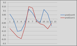
Proof that fMRI data is (mostly) crap

These are timecourses extracted from two different conditions, helpfully labeled "pred2corr0" and "pred2corr1". When we took a contrast of pred2corr0 and compared it to pred2corr1, we got a positive value. However, here's what happened: The peaks of the HRF (represented here by the timepoints under the "3" in the x-axis, which translates into 6 seconds (3 scans of 2 seconds each = 6 seconds), representing the typical peak of the HRF after the onset of a stimulus) for both conditions were negative. It just happened that the peak for the pred2corr1 condition was more negative than that of pred2corr0, hence the positive contrast value.

2) If you have selected "Temporal Derivative" for all of your regressors, then every other column will represent an estimate of what the temporal derivative should look like. Adding a temporal derivative has the advantage of accounting for any potential lags in the onset of the HRF, but comes at the cost of a degree of freedom, since you have something extra to estimate.

3) After the model is set up and you click on the "Efficiency" tab, you will see two sections. The section on the left represents the correlation between regressors, and the section on the right represents the singular value decomposition eigenvalue for each condition.

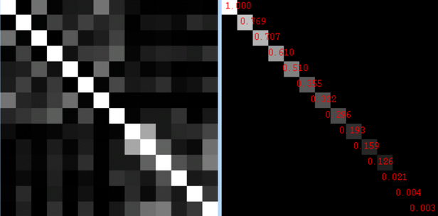
What is an eigenvalue? Don't ask me; I'm just a mere cognitive neuroscientist.

For the correlations, brighter intensities represent higher correlations. So, it makes sense that the diagonal is all white, since each condition correlates with itself perfectly. However, it is the off-diagonal squares that you need to pay attention to, and if any of them are overly bright, you have a problem. A big one. Bigger than finding someone you loved and trusted just ate your Nu-...but let's not go there.

As for the eigenvalues on the right, I have yet to find out what range of values represent safety and which ones represent danger. I will keep looking, but for now, it is probably a better bet to do design efficiency estimation using a package like AFNI to get a good idea of how your design will hold up under analysis.


That's it. A few more videos will be uploaded, and then the beginning user should have everything he needs to get started.

FSL Tutorial 2: FEAT (Part 1)

A new tutorial about FEAT is now up; depending on how long it takes to get through all of the different tabs in the interface, this may be a three-part series. In any case, this will serve as a basic overview of the preprocessing steps of FEAT, most of which can be left as a default.

The next couple of tutorials will cover the set up of models and timing files within FSL, which can be a little tricky. For those of you who have stuck with it from the beginning (and I have heard that there are a few of you out there: Hello), there will be some more useful features coming up, aside from reviewing the basics.

Eventually we will get around to batch scripting FEAT analyses, which can save you several hours of mindless pointing and clicking, and leave you with plenty of time to watch Starcraft 2 replays, or Breaking Bad, or whatever it is kids watch these days.

FSL Tutorial 0: Conversion from DICOM to NIFTI

After publishing my last tutorial, I realized that I should probably take a step back and detail how to convert raw scanner images into something that can be used as FSL. This latest walkthrough will show you how to download MRIcron and use one of its tools, dcm2nii, to convert raw scanner image formats such as DICOM or PAR/REC to nifti, which can be used by almost all fMRI software analysis packages.

Note: I've been using Camtasia Studio to make these screencasts, and so far I have been very happy with it. The video editor is simple and intuitive, and making videos isn't too difficult. It runs for $99, which is a little pricey for a screencast tool, but if you're going to be making them on a regular basis and doing tutorials, I would recommend buying it.

Repost: Why Blogs Fail

Pictured: One of the reasons why blogs fail

Blogger Neuroskeptic recently wrote a post about why blogs fail, observing what divides successful from unsuccessful blogs, and why the less successful ones ultimately stop generating new content or disappear altogether. Reading this made me reflect on why I started this in the first place; initially it was to write down, in blog-form, what I saw and heard at an AFNI workshop earlier this spring. Since then, I tried to give it a more coherent theme, by touching upon some fMRI methodology topics that don't get as much attention as they deserve, and creating a few walkthroughs to help new students in the field get off the ground, as there isn't much out there in the way of interactive videos showing you how to analyze stuff.

Analyzing stuff, in my experience, can be one of the most intimidating and paralyzing experiences of a graduate student's career; not because of laziness or incompetence, but because it is difficult to know where to start. Some of the obstacles that hinder the analysis of stuff (e.g., common mistakes involving experiment timing, artifacts that can propagate through an entire data set, not having a method for solving and debugging scripting errors) do not need to be repeated by each generation, and my main objective is to point out where these things can happen, and what to do about them. Of course, this blog contains other topics related to my hobbies, but overall, the theme of how to analyze stuff predominates.

In light of all of this, here is my pact with my readers: This blog will be updated at least once a week (barring any extreme circumstances, such as family emergencies, religious observations, or hospitalization from Nutella overdose); new materials, such as walkthroughs, programs, and instructional videos, will be generated on a regular basis; and I will respond to any (serious) questions posted in the comments section. After all, the reason I take any time out of my busy, Nutella-filled day to write any of this content is because I find it interesting and useful, and hope that somebody else will, too.

Chopin: Nocturne in E-flat Major

This is probably one of the best-known and best-loved out of all Chopin's nocturnes - rightly so. Although it has been overplayed to death, and although several performances suffer from excruciatingly slow tempi, no one can deny its elegance and charm.

The architecture is straightfoward enough: an A section which repeats, followed by a B section, then A again, then B, and a coda, in a form technically known as rounded binary. Chopin's genius lies in keeping the same harmonic foundation in each repeated section while progressively ornamenting the melody, finding ways to keep it fresh and exciting every time it returns. Finally, elements of both themes in the A and B sections are combined into a wonderful coda (listen for them!), becoming increasingly agitated until reaching an impassioned dominant, prepared by a c-flat anticipation held for an almost ridiculous amount of time.

Almost - Chopin, as well as Beethoven, is a master at reaching the fine line separating drama and melodrama, pathos and sentimentality, without going over the edge. The famous cadenza - a four-note motif marked senza tempo during which time stands still - repeats faster and faster, more and more insistent, until finally relenting, and finding its way back to a tender, emotional reconciliation with the tonic.

Enjoy!

FSL Tutorial: Part 1 (of many)

I recently started testing out FSL to see if it has any advantages over other fMRI analysis packages, and decided to document everything on Youtube as I go along. The concepts are the same as any other package (AFNI, SPM, etc), but the terminology is slightly different, and driving it from the command line is not as intuitive as you would think. Plus, they use a ton of acronyms for everything, which, to be honest, kind of pisses me off; I don't like it when they try to be cute and funny like that. The quotes and sonnets generated by AFNI after exiting the program, however, are sophisticated and endearing. One of my favorites: "Each goodbye makes the next hello closer!"

In any case, here is the first, introductory tutorial I made about FSL. I realized from searching around on Youtube that hardly any fMRI analysis tutorial videos exist, and that this is a market that sorely needs to be filled. A series of walkthroughs and online lessons using actual data, in my opinion, would be far more useful at illustrating the fundamentals of fMRI data analysis than only having manuals (although those are extremely important as well, and I would recommend that anyone getting started in the field read them so that they can needlessly suffer as I did).

I will attempt to upload more on a regular basis, and start to get some coherent lesson plan going which allows the beginner to get off the ground and understand what the hell is going on. True story: It took me at least three years to fully comprehend what a beta weight was. Three years. I'm not going to blame it all on Smirnoff Ice, but it certainly didn't help.

Note: I suggest hitting fullscreen mode and viewing at a higher resolution (360p or 480p) in order to better see the text in the terminal window.

Also, the example data for these tutorials can be found here.