Updated Functional Connectivity Tutorial using AFNI

As part of a new course in neuroimaging methods at Haskins Laboratories, I've begun updating videos on topics such as functional connectivity, context-dependent correlations, and how to accept bribes as a reviewer. The first topic we've covered is resting-state functional connectivity, a sophisticated-sounding name designed to make the subject think he is doing something of immense scientific importance by lying still and doing nothing, when in reality it's to distract him while we find out how to hell to hook up the experimental laptop.

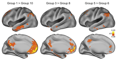
Aside from its usefulness as a stall tactic, resting-state connectivity can also reveal resting-state networks, or correlations between the signal of distant regions of the brain. This provides clues to how structural connectivity - i.e., white matter connections - interact with the BOLD signal, as well as whether differences in resting-state connectivity is a marker for mental disorders such as Alzheimer's or schizophrenia.

The following video takes you step-by-step through functional connectivity analysis, using an online dataset from openfmri.org. One major change from my previous tutorials is condensing all the information into one long video, and providing time markers for each segment in the "Show More" box. This way the viewer can jump around to the information that they need, without having to keep track of several different videos detailing different steps. I hope it's an improvement, and I would like to get feedback.

I've also posted the lecture on resting-state analysis given at Haskins Laboratories on November 3rd. You won't learn much new here that isn't in the video above, but it does have more information. For most of the lecture you can only see the top of my head bobbing around, but that's OK. Eyes on the slides, not the hair.

Exercises:

1. Set the errts dataset as the underlay, and select "Graph". From the "Opt" menu, select "Write Center." Rename the output 1D file, and use 1dplot to see the timecourse. This can be used as a seed for another connectivity analysis.
2. Other resting state networks include the somatosensory network, the visual network, and the language network. Research one of these networks, determine where the hubs are, and run a resting state analysis on a seed placed in that hub.
3. Run correlations for a group of subjects, convert to z-scores, and do a second-level t-test using uber_ttest.py.
4. Modify the afni_proc.py script to apply 3dRSFC to your data (see Example 10b in afni_proc.py -help)

Resting-State Functional Connectivity Analysis, Part II: Setting Up Your Analysis

Once you have downloaded the KKI dataset discussed in the last resting-state post, you have most of what you need, sacrificial undergraduate RA notwithstanding. Also, as I mentioned, we will be using AFNI for this, specifically AFNI's uber_subject.py script which includes an option for preprocessing and analyzing resting-state data.

First, type uber_subject.py from your terminal to open up the GUI (rhymes with "whey"), and select the resting-state option from the preprocessing selections. This will automatically fill in a series of preprocessing steps which our AFNI overlords, in their wisdom, have decided is best for resting-state analyses. Of course, you can change this, but that would be an unbelievably stupid decision, on par with doing something like asking out your girlfriend's sister.

Notice that with resting-state experiments, we avoid several of the annoying, persnickety details endemic to typical FMRI experiments, such as having to actually design an experiment. You simply place the subject inside the scanner, set the scanner to 350 degrees, and leave it for ten minutes. When you come back, you will have a slightly charred piece of carbon that used to be a human being. After framing someone else, such as your FMRI technician, you should then realize that you are simply not cut out for actually carrying out a resting-state scan, and download someone else's data instead from the Internet like I recommended in the first place.

Notice that much of the preprocessing and setting up the design matrix is the similar to usual FMRI analyses. However, there is an important difference in the design matrix setup, because you do not have any tasks or events to model. Instead, the only things you need to model are potential sources of noise, which may include heart rate or respiration data, if you have it, and always motion data, since this can be an insidious confound in any FMRI analysis, but particularly for resting-state analyses.

The upshot of all this is that, whereas in a traditional FMRI analysis AFNI saves the beta estimates and contrasts to a statistics dataset and everything else that wasn't modeled into an error or residual dataset (usually labelled "errts+orig"), in resting-state analyses we are interested in everything that wasn't explicitly modeled - in other words, we will want to focus on what gets output to the errts+orig dataset, since that will contain the timecourses of voxel activity that we are interested in. You can then place ROIs or other seed regions within that dataset, and generate correlation maps from those seed regions.

In the next chapter of the series, we will look more closely at converting these correlation values into z-maps for comparison across groups, as well as where to find more undergraduate RAs if the ones who were working in your lab have already been burnt as offerings to the FMRI gods.

Introduction to Resting-State Functional Connectivity Analysis: You Can Do It! (Maybe)

A while ago I promised to provide a series of tutorials on resting-state connectivity, and I'm happy to announce the first part after a brief delay of, give or take, fourteen months. But in my defense, I wanted to wait until I had everything well prepared and ready to go, by which I mean until I had a new suit, which, obviously, is a critical part of the education process.

For this series, in order to follow along I recommend downloading resting-state data from the ABIDE website, which collects resting-state data from autistic subjects and controls. The end result will be a simple comparison of resting-state networks across both populations, which, although the interpretation of such results has a large farrago of its own issues, should provide a solid platform from which to launch your own resting-state analyses. We will be using AFNI for this demonstration, although in the future I may include an identical analysis using FSL.

First, you need to jump through the usual administrative hoops in order to download the dataset. This involves a simple series of steps, such as registering as a member, filling out a form with your username and password, and immolating a virginal undergraduate RA. The resulting aroma will summon the resting-state data, which can then be downloaded to your computer.

First, register at the NITRC website: http://www.nitrc.org/account/register.php
Two, request access from the following link: http://fcon_1000.projects.nitrc.org/indi/req_access.html
Last, go to the ABIDE website and download a resting-state dataset (I am using data from the Kennedy Krieger Institute): http://fcon_1000.projects.nitrc.org/indi/abide/

As for finding and sacrificing the virginal undergraduate RA, you're on your own.

Creating Functional Connectivity Maps in AFNI (Second Step on the Road Towards Glory)

Having used 3dSynthesize to create a dataset with the effects of no interest, we are now ready to subtract those effects from the dataset that went into 3dDeconvolve; for you players using the AFNI_data6 tutorial data, this is the all_runs.FT+orig dataset. We can use 3dcalc for this operation:

3dcalc -a all_runs.FT+orig -b effectsNoInterest+orig -expr 'a-b' -prefix cleanData+orig

This will create a time series with all the drift correction and motion parameter schmutz subtracted out and cast into the pit. What is left over will be signal untainted by motion or drift effects, which we can then use to generate a seed time series.

Before that, however, there is the additional step of warping our data to a template space (such as MNI or Talairach). Assuming you have already warped your anatomical dataset to a template space either manually or using @auto_tlrc, and assuming that there is already good alignment between your anatomical and functional data, you can use the command adwarp:

adwarp -apar anat_final.FT+tlrc -dpar cleanData+orig -dxyz 3 -prefix EPI_subj_01

(Note: There are better ways to do warping, such as the warping option built into align_epi_anat.py (which calls upon @auto_tlrc), but for pedagogical purposes we will stick with adwarp.)

Once this is done, all we need to do is select a seed region for our functional connectivity analysis. This could be a single voxel, a region of interest that averages over an entire area of voxels, or a region selected based on a contrast or an anatomical landmark; it depends on your research question, or whether you want to mess around and do some exploratory analyses. For now, we will use a single voxel using XYZ coordinates centered on the left motor cortex (note that, in this coordinate system, left is positive and posterior is positive):

3dmaskdump -noijk -dbox 20 19 53 EPI_subj_01+tlrc > ideal_ts.1D

Because 3dmaskdump outputs a single row, we will need to transpose this into a column:

1dtranspose ideal_ts.1D LeftMotorIdeal.1D

After you have output your ideal timeseries, open up the AFNI viewer and make sure that what was output matches up with the actual timeseries. In this example, set EPI_subj_01+tlrc as an underlay and right click in the slices viewer to jump to XYZ coordinates of 20, 19, 53; open up the timeseries graph as well, and scroll to the first time point. Does the value there match up with the first entry of your ideal time file? If not, you may have mis-specified the voxel you wanted, or you are using a different XYZ grid than is displayed in the upper left corner of the AFNI viewer. If you run into this situation, consult your local AFNI guru; if you don't have one of those, well...

In any case, we now have all the ingredients for the functional connectivity analysis, and we're ready to pull the trigger. Assemble your materials using 3dfim+ (which, as far as I can understand, stands for "functional intensity map," or something like that):

3dfim+ -polort 3 -input EPI_subj_01+tlrc -ideal_file LeftMotorIdeal.1D -out Correlation -bucket Corr_subj01

You will now have a dataset, Corr_subj_01+tlrc, which is a functional connectivity map between your seed region and the rest of the brain. Note that the threshold slider will now be in R values, instead of beta coefficients or t-statistics; therefore, make sure the order of magnitude button (next to the '**' below the slider) is 0, to restrict the range between +1 and -1.

The last step is to convert these correlation values into z-scores, to reduce skewness and make the distribution more normal. This is done through Fisher's R-to-Z transformation, given by the formula z =  (1/2) * ln((1+r)/(1-r)). Using 3dcalc, we can apply this transformation:

3dcalc -a Corr_subj01+tlrc -expr 'log((1+a)/(1-a))/2' -prefix Corr_subj01_Z+tlrc

Those Z-maps can then be entered into a second-level design just like any other, using 3dttest+ or some other variation.

Sanity check: When viewing the correlation maps, jump to your seed region and observe the r-value. It should be 1, which makes sense given that this was the region we were correlating with every other part of the brain, and correlating it with itself should be perfect.

Like me.

Introduction to Functional Connectivity

It seems as though everyone these days wants to do something more than just the same old standard mass univariate analyses. And why not? Given the embarrassment of riches we have with any FMRI dataset - literally thousands upon thousands of voxels in just a single image, like some gargantuan godsized Rubik's Cube with as many interlocking blocks as there are grains of sand on the beach - it is too tempting not to. In each dataset - hundreds of thousands of voxels. In each experiment - millions. In a lab - tens of millions. In a university - billions. And on and on. As Jeeves would say: The mind boggles, sir.

With so much data at our disposal, one naturally wants to do more sophisticated analyses and test for more interesting types of interactions; and this impulse becomes even stronger among the neurotic academic who has to make things much more complex then they really have to be. To see whether there are any special affinities between different regions of the brain, as it were. Due to the incredibly high number of connections within it, more complex analysis of the interactions between the signals of the voxels themselves becomes compelling - and one of the ways to do this is through a technique called functional connectivity.

All functional connectivity is, in its most basic form, is calculating the correlation between the timeseries of different voxels. The reference timecourse is determined entirely by the investigator; it can be a single peak voxel within a cluster defined by a contrast, it can be an average timecourse across an entire blob of contiguous voxels, or it can be a voxel chosen on the basis of its anatomical location. However it is chosen, this reference timecourse is compared against every other voxel in the brain, and a correlation coefficient computed to measure the similarity between the timecourses. In other words, does this voxel's timeseries, picked from an arbitrary point on the left side of the brain:

Match up well with another voxel picked from the right side of the brain?

Reference timecourse overlaid in red, above the comparison voxel's timecourse in black.

And this same procedure is applied for every other voxel as well.

However, it is worth noting that the name "Functional Connectivity" is misleading at best. Really what it is is a simple correlation analysis, often more appropriately called a bivariate correlation analysis. There is no connectivity to speak of in this kind of analysis; we merely operate under the assumption voxels showing similar timecourses might - might - be connected somehow. But even this is a somewhat laughable assumption to make. No temporal delay is really considered, and no directionality can be inferred.

With this I come to a conclusion and pronounce my judgment. I condemn the name functional connectivity; I raise against this wretched misnomer the most terrible of all the accusations that an accuser ever uttered. It is, to me, the highest of all conceivable corruptions; it seeks to work the ultimate corruption, the worst possible corruption. The name "functional connectivity" has left nothing untouched by its depravity; it has turned every value into worthlessness, and every truth into a lie, and every integrity into vileness of soul. Let any one dare to speak to me of its "scientific" blessings!

Parasitism is the only practice of those who call it so; with its anemic and "connectivity" ideals, sucking all the blood, all the love, all the hope out of life; the will to negate all reality; the word "connectivity" as the mark of recognition for most subterranean conspiracy ever heard of - against health, beauty, well-being, intellect, graciousness of soul - against life itself. This eternal indictment against the name functional connectivity I shall write upon all walls, wherever walls are to be found - I have letters that even the blind will be able to see.

I call that name the one great curse, the one great intrinsic depravity, for which no means are venomous enough, or secret, subterranean and small enough; I call it the one immortal blemish upon the human race.



Of course, if you do want to do a real connectivity analysis, that requires some more steps. We will get to all of that later; but first things first. Here are some of the basics.

One Weird Trick to Boost Brain Connectivity

Answer: Take an LSAT course.

At least, that seems to contribute to changes in resting-state functional connectivity between distinct brain regions, according to a new study in the Journal of Neuroscience by Mackey et al (2013). The researchers took two groups of pre-law students and divided them into a training group, which was taking an LSAT prep course, and a control group, which intended to take the LSAT but was not enrolled in the prep course. After matching the subjects on demographics and intelligence metrics, functional connectivity was measured during a resting state scan (which, if you remember from a previous post, is a measure of correlation between timecourses between regions, rather than physical connectivity per se).

Taking the LSAT prep course was associated with increased correlations between the rostro-lateral prefrontal cortex (RLPFC; a few centimeters inside your skull if you take your finger and press it against your forehead just to the lateral side of your eye) and regions of parietal cortex (located more to the rear of your skull, slightly forward and lateral of the bump in the back of your head). The RLPFC seems to help integrate abstract relations, such as detecting flaws in your spouse's arguments, while the parietal cortex processes individual relations between items. Overall, when they combine forces, as shown by a concomitant increase in functional connectivity and test scores, your LSAT skills become unstoppable.

The parietal cortices and striatal regions, particularly the caudate and putamen nuclei, showed a stronger coupling as a result of taking the prep course; presumably because of the strong dopaminergic inputs from the basal nuclei and striatum, which emit bursts of pleasure whenever you make a breakthrough in reasoning or learning. This should come as no surprise to classical scholars, as Aristotle once observed that the two greatest peaks of human pleasure are 1) thinking, and 2) hanky-panky. (Or something like that.)

Taken to the extreme, these results suggest efficient ways to manufacture super-lawyers, or at least to strengthen connectivity between disparate regions, and alter resting state dynamics. This touches on the concept of neuroplasticity, which suggests that our brains are adaptive and malleable throuhgout life, as opposed to traditional views that cognitive stability and capacity plateaus sometime in early adulthood, and from there makes a slow decline to the grave. Instead, regularly engaging your thinking muscles and trying new cognitive tasks, such as mathematics, music, and fingerpainting, as well as grappling with some of the finest and most profound philosophical minds humanity has produced - Kant, Kierkegaard, Hegel, Nietzsche, Andy's Brain Blog, et alia - will continue to change and transmogrify your brain in ways unimaginable and calamitous beyond reckoning.


Thanks to Simon Parker. (LSAT professors hate him!)

Head Motion and Functional Connectivity

Yesterday as I was listening to a talk about diffusion tensor imaging, a professor asked about the influences of head motion on DTI data, and whether it could lead to spurious effects. Another professor vigorously denied it, stating that it was much more of a problem for bread and butter FMRI analyses, and in particular resting state functional connectivity analyses. At one point he became so animated that his monocle fell off, his collar stud came undone, and eventually he had to be physically restrained by the people sitting next to him. It was then that I knew that I should pay heed, for it is unlikely that a scientist becomes highly excited and talkative over matters that are trivial; in short, I could sense that he was talking about something important.

I have done few functional connectivity analyses in my brief life, but what I understand about them is this: You take the timecourse of one voxel - or the average timecourse over a group of voxels, also known as a "seed" - and then compare that timecourse with the timecourse of every other voxel in the brain. (When I speak of timecourses, I mean the sampled signal over time.) If it is a good fit - in other words, if there is a significantly high correlation between the timecourses - then we say that the two regions are functionally connected. This is a bit of a misnomer, as we cannot make any direct inferences about any "real" connectivity from two correlated timecourses; but it can serve as a good starting point for more sophisticated analyses, such as psychophysiological interactions (PPI; also known as context-dependent correlations) which measure changes in functional connectivity as a function of task context. For example: Does the timecourse correlation between cognitive control regions and reward-related areas change depending on whether the subject is instructed to upregulate or downregulate their gut reactions to rewarding stimuli?

One of the most popular variations of functional connectivity is something called resting state functional connectivity (rsFC), where a subject is simply instructed to relax and listen to Barry Manilow* while undergoing scanning. Functional connectivity maps are then calculated, and usually a comparison is made between a control group and an experimental or patient group, such as schizophrenics. For us FMRI researchers, this is about as close as we can get to simulating a person's natural environment where they would be relaxing and thinking about nothing in particular; except that they're in an extremely tight-fitting, noisy tube, and unable to move in any direction more than a few millimeters. Other than that, though, it's pretty normal.

These types of experiments have become all the rage in recent years, with several studies claiming to have found meaningful resting-state differences between healthy controls and several different patients populations such as schizophrenics, depressives, Nickelback fans, and drug addicts. However, a few publications have called into question some of these results, stating that many of these differences could be due to head motion. As we've talked about before, head motion can be a particularly insidious confound in any experiment, but it is especially troublesome for functional connectivity analyses. This can arise due to systematic differences between control and patient populations that are possibly confounded with motion. Take, for example, an experiment contrasting young versus older populations. Older populations are known to move more, and any observed differences in functional connectivity may be due solely to this increased motion, not underlying neural hemodynamics.

A study by Van Dijk, Sabuncu, & Bruckner (2012) looked at this in detail by scanning over a thousand (!) subjects, and binning them into ten groups based on increasing amounts of motion (e.g., group 1 had the least amount of motion, while group 10 had the most motion). The authors found decreased functional connectivity in the "default network" of the brain - usually referring to the functional connectivity between the medial prefrontal cortex and retrosplenial cingulate cortex -, decreased connectivity in the frontal-parietal network, and slightly increased local connectivity among clustered voxels, simply based on motion alone. (Keep in mind that each bin of subjects were matched as closely as possible on all other demographic measures.) Furthermore, even when comparing bins of subjects closely matched for motion (e.g., bins 5 and 6), small but significant differences in functional connectivity were seen.

Figure 3 from Van Dijk et al (2012). Functional connectivity among different networks measured as a function of head motion. Both linear and nonlinear (quadratic) terms were modeled to fit the data.

Figure 4 from Van Dijk et al (2012). Note the comparison on the far right between groups 5 and 6; the mean motion difference between these two groups is a few thousandths of a millimeter, but noticeable functional connectivity differences are still seen between the two groups.

Lastly, a subset of subjects were rescanned in order to see whether motion was reliable; in other words, if a subject that moved a large amount on one day had the same tendency to move a large amount on the next day. A clear correlation was found between scanning subjects, suggesting that motion might need to be treated as a trait or individual difference, just like any other.

Figure 5 from Van Dijk et al (2012). There is a robust correlation between the movement of scanning sessions, even with the outliers removed (marked in diamonds).

So, what to do? A few recommendations are to match subjects for motion, correct motion prospectively (Ward et al, 2000), and regress out motion when performing a group-level analysis, as you would any other covariate. Apparently traditional methods of motion correction on a subject-by-subject basis are not enough, and increasing awareness of the pitfalls of between-subject motion is important for evaluating current functional connectivity analyses, and for conducting your own experiments.

This study hit me in the face like a wet mackerel since I am beginning to investigate a recent AFNI tool, 3dReHo, to do local functional connectivity analyses for publicly available datasets on the ABIDE website. However, as far as I can tell, motion limits were not used as exclusionary criteria, which may be a possible confound when examining, say, autistic children to controls. More to come soon. Or not.



*I Don't Want to Walk Without You

Resting State Functional Connectivity Database

For those of you not in the know, there is a gimundo FMRI database comprising resting state datasets from research laboratories all over the world. (Meaning the United States, Belgium, Ireland, and the Netherlands.) Scanning parameters and sample features are included with each dataset, making it straightforward to download and analyze entire datasets with relative ease. This is my first time doing resting state functional connectivity analysis, as I have never before collected a dataset using this technique, and I will be sure to document my progress as I go along.


Thanks to Omar Maximo, who can dunk a basketball literally AND figuratively.

Let's Talk about Masks (Live Video)

I've been experimenting more with Camtasia, and I've uploaded a new video showing how masks are drawn on an actual human, rubber brain, which involves the use of R studio, Excel, and colored pens. My hope is that this makes the learning experience more interactive; in addition, you get to see what my mug looks like.

Unix for Neuroimagers: Shells and Variables

First, a few updates:

1) We just finished our first week of the semester here, and although things haven't been too busy, it may be a couple of weeks before I get back on a steady updating schedule. I'll do what I can to keep dropping that fatty knowledge on the regular, and educating your pale, soy-latte-white, Famous Dave's BBQ-stained faces on how to stay trill on that data and stack that cheddah to the ceiling like it's your job. And if you got one of those blogs dedicated to how you and your virgin-ass Rockband-playing frat brothers with names like Brady and Troy and Jason eating those cucumber salad sandwiches or whatever and you drop a link to this site, I'll know it. You show me that love, and I show it right the hell back.

2) While you're here, how about you donate a piece of that stack to the American Cancer Society. I mean, damn; I'm out there seven days a week on those roads, sweating and suffering, but you - you're at work procrastinating again, wringing your snow-bunny white hands over whether you should drop out of graduate school or just toughen it out and graduate in eight years, and while you're at it possibly take a swipe at that new Italian breezey who just entered the neuroscience program. Donate first, worry about those problems later.

3) We got another performance for you all this November, including Schumann's Adagio and Allegro for cello and piano, Resphigi's Adagio con Variazioni, and the Debussy cello sonata. Time and location TBA. Also, more music videos will be uploaded soon, but while you're waiting, you can listen to the latest Mozart Fantasie in D Minor, which has proved one of my most popular videos to date; last I checked, it had 57 views, which I think qualifies for viral status. We goin' worldwide, baby! World-WIDE!!

4) AFNI tutorials are next on the docket, after wrapping up the intro Unix tutorials for neuroimagers, and possibly doing a couple more FSL tutorials on featquery, FSL's ROI analysis tool. Beyond that, there isn't much else I have to say about it; now that you've mastered the basics, you should be able to get the program to jump through whatever hoops you set up for it and to do whatever else you need. There are more complex and sophisticated tools in FSL, to be sure, but that isn't my focus; I will, on the other hand, be going into quite a lot of details with AFNI, including how to run functional connectivity and MVPA analyses. It will take time, but we will get there; as with the FSL tutorials, I'll start from the bottom up.


Anyway, the latest Unix tutorial covers the basics on shells and variables. Shells are just ways of interfacing with the Unix OS; different shells, such as the t-shell (tcsh) and bash shell, do the same thing, but have different syntax and different nomenclature for how they execute commands. So, for example, an if/else statement in the t-shell looks different from a similar statement in the bash shell.

Overall, there's no need to worry too much about which shell you use, although AFNI's default is tcsh, so you may want to get yourself used to that before doing too much with AFNI. I myself use tcsh virtually all of the time, except for a few instances where bash is the only tool that works for the job (running processes on IU's supercomputer, Quarry, comes to mind). There are lots of tcsh haters out there for reasons that are beyond me, but for everything that I do, it works just fine.

As for variables, this is one of the first things you get taught in any intro computer science class, and those of you who have used other software packages, such as R or Matlab, already know what a variable is. In a nutshell, a variable is a thing that has a value. The value can be a string, or a letter, or a number, or pretty much anything. So, for example, when I type in the command

set x=10

in the t-shell, the variable is x, and the value is now 10. If I wish to extract the value from x at any time, I prepend a dollar sign ('$') to it, in order to tell Unix that what follows is a variable. You can also use the 'echo' command to dump the value of the variable to the standard output (i.e., your terminal). So, typing

echo $x

returns the following:

10

which is the value that I assigned to x.

From there, you can build up more complicated scripts and, by having the variable as a placeholder in various locations in your script, only have to change the value assigned to it in order to change the value in each of those locations. It makes your programming more flexible and easier to read and understand, and is critical to know if you wish to make sense of the example scripts generated by AFNI's "uber" scripts.

With all of the tutorials so far, you have essentially all of the fundamentals you need to operate FSL. Really, you only need to understand how to open up a terminal and make sure your path is pointing to the FSL binaries, but after that, all you need to do is understand the interface, and you can get by with pointing and clicking. However, a more sophisticated understanding is needed for AFNI, which will be covered soon. Very soon. Patience, my pretties.