Duration Regressors with fMRI

This subject was brought to my attention by a colleague who wanted to know whether parametric modulation or duration modulation was a better way to account for RT effects. While it can depend on the question you are trying to answer, often duration modulation (referred to here as a "variable epoch model") works best. The following highlights the different approaches for modeling trials which involve a period of decision-making or an interval between presentation of a stimulus and the resulting response.


Over the past few years there has been a renewed interest in modeling duration in fMRI data. In particular, a methods paper by Grinband and colleagues (2008) compared the effects of modeling the duration of a trial - as measured by its reaction time (RT) - against models which used RT as a parametric modulator and against models which did not use RT at all. The argument against using RT-modulated regressors was that, at short time intervals (i.e., less than four seconds), using an impulse function was a good approximation to the resulting BOLD signal (cf. Henson, 2003).

Figure depicting relationship between stimulus onset, BOLD response, and underlying neural activity. Red lines: activity associated with punctate responses (e.g., light flashed at the subject). Blue lines: Activity associated with trials of unequal duration (e.g., decision-making).

However, for a few investigators, such assumptions were not good enough. To see whether different models of RT led to noticeable differences in BOLD signal, Grinband et al (2008) examined four types of modeling:

1. Convolving the onset of a condition or response with the canonical HRF (constant impulse model);
2. Separately modeling both the main effect of the condition as well as a mean-centered parametric modulator - in this case RT (variable impulse model);
3. Binning each condition onset into a constant amount of time (e.g., 2 seconds) and convolving with the canonical HRF (constant epoch model); and
4. Modeling each event as a boxcar function equal to the length of the subject's RT (variable epoch model).

Graphical summary of models from Grinband et al (2008). Top: Duration of cognitive process as indexed by reaction time. Constant Impulse:  Onset of each event treated as a punctate response. Constant Epoch: Onset of each event convolved with boxcar function of constant duration. Variable Impulse: Punctate response functions modulated by mean-centered parameter (here, RT). Variable Epoch: Each event modeled by boxcar of duration equal to that event's RT.

Each of these models was then compared using data from a decision-making task in which subjects determined whether a line was long or short. If this sounds uninteresting to you, you have obviously never done a psychology experiment before.

The authors found that the variable epoch model - in other words, convolving each event with a boxcar equal to the length of the subject's RT for that trial - captured more of the variability in the BOLD response, in addition to reducing false positives as compared to the other models. The variable epoch model also dramatically increased sexual drive and led to an unslakeable thirst for mindless violence. Therefore, these simulations suggest that for tasks requiring time - such as decision-making tasks - convolution with boxcar regressors is a more faithful representation of the underlying neuronal dynamics (cf. the drift-diffusion model of Ratcliff & McKoon, 2008). The following figures highlight the differences between the impulse and epoch models:

Comparison of impulse models and epoch models as depicted in Grinband et al (2008). A) For impulse models, the shape remains constant while the amplitude varies; for epoch models, increasing the duration of a trial leads to changes in both shape and amplitude. B) Under the impulse model, increasing the duration of a stimulus or cognitive process (as measured by RT) leads to a reduction in explained variance.

Figure from Grinband et al (2008) showing differential effects of stimulus intensity and stimulus duration. Left: Increasing stimulus intensity has no effect on the time to peak of the BOLD response. Right: Increasing stimulus duration (or the duration of the cognitive process) leads to a linear increase in the time for the BOLD response to peak.

One caveat: note well that both parametric modulation and convolution with boxcar functions will account for RT-related effects in your data; and although the Grinband simulations establish the supremacy of boxcar functions, there may be occasions that warrant parametric modulation. For example, one may be interested in the differences of RT modulation for certain trial types as compared to others; and the regressors generated by parametric modulation will allow the researcher to test them against each other directly.

AFNI Tutorial: 3dTcat

AFNI's 3dTcat is used to concatenate datasets. For example, after performing first- and second-level analyses, you may want to join several datasets together in order to extract beta weights or parameter estimates across a range of subjects. Conversely, you may want to create a dataset that contains only a subset of the sub-briks of another dataset. This function is covered in the following AFNI video tutorial.

(N.B.: In AFNI Land, a sub-brik represents an element of an array. With runs of fMRI data, this usually means that each sub-brik is a timepoint; that is, an individual volume. When 3dTcat is used to concatenate sub-briks from multiple datasets containing beta weights, the resulting dataset is a combination of parameter estimates from different subjects, and it falls to you to keep track of which beta weight belongs to which subject. More on this at a later time.)

3dTcat is straightforward to use: Simply supply a prefix for your output dataset, as well as the range of sub-briks you wish to output. A typical 3dTcat command looks like this:

3dTcat -prefix r01_cat r01+orig'[2..$]'

This command will create a new dataset called "r01_cat", consisting of every sub-brik in r01+orig except for sub-briks 0 and 1 (recall that most AFNI commands associate 0 with the first element in an array). The '..' means "every sub-brik between these two endpoints", and the '$' sign represents the last element in the array (in this example, 205, as there are 206 timepoints; recall again that since 0 is regarded as a timepoint, we subtract 1 from the total number of timepoints to get the last element of the array).

Other patterns can be used as well, such as selecting only certain sub-briks or selecting every other sub-brik. These examples are taken from the help of 3dTcat:

  fred+orig[5]                     ==> use only sub-brick #5
  fred+orig[5,9,17]                ==> use #5, #9, and #17
  fred+orig[5..8]     or [5-8]     ==> use #5, #6, #7, and #8
  fred+orig[5..13(2)] or [5-13(2)] ==> use #5, #7, #9, #11, and #13

As emphasized in previous posts, you should check your data after running a command. In the video tutorial, we ran 3dTcat on a dataset which had 206 volumes; the resulting dataset chopped off the first two volumes, reducing the volumes in the output dataset to 204. You can quickly check this using 3dinfo with the -nt command, e.g.:

3dinfo -nt r01_cat+orig

This command will return the number of timepoints (or sub-briks, or elements) in the dataset. This can be a useful tool when you wish to execute conditional statements based on the number of sub-briks in a dataset.

More information on the evils of pre-steady-state volumes can be found here.

AFNI Tutorial: to3d

In the beginning, a young man is placed upon the scanning table as if in sacrifice. He is afraid; there are loud noises; he performs endless repetitions of a task incomprehensible. He thinks only of the coercively high amount of money he is promised in exchange for an hour of meaningless existence.

The scanner sits in silent judgment and marks off the time. The sap of life rushes to the brain, the gradients flip with terrible precision, and all is seen and all is recorded.

Such is the prologue for data collection. Sent straight into the logs of the server: Every slice, every volume, every run. All this should be marked well, as these native elements shall evolve into something far greater.

You will require three ingredients for converting raw scanner data into a basic AFNI dataset. First, the number of slices: Each volume comprises several slices, each of which measures a separate plane. Second, the number of volumes: Each run of data comprises several volumes, each of which measures a separate timepoint. Third, the repetition time: Each volume is acquired after a certain amount of time has elapsed.

Once you have assembled your materials, use to3d to convert the raw data into a BRIK/HEAD dataset. A sample command:

to3d -prefix r01 -time:zt 50 206 3000 alt+z *000006_*.dcm

This command means: "AFNI, I implore you: Label my output dataset r01; there are 50 slices per volume, 206 volumes per run, and each volume is acquired every 3000 milliseconds; slices are acquired interleaved in the z-direction; and harvest all volumes which contain the pattern 000006_ and end in dcm. Alert me when the evolution is complete."

More details and an interactive example can be found in the following video.

Disclaimers

Yesterday I was surprised to find AFNI message boards linking to my first blog post about AFNI. I felt as though the klieg lights had suddenly been turned on me, and that hordes of AFNI nerdlings would soon be funneled into this cramped corner of cyberspace. If you count yourself among their number, then welcome; I hope you enjoy this blog and find it useful.

However, there are a few disclaimers I should state up front:

1. I do not work for AFNI; I am merely an enthusiastic amateur. If you post any questions either on this blog or on Youtube I will be more than willing to answer them. However, if it is something over my head that I can't answer, then I will suggest that you try the official AFNI message board - it is policed 24/7 by the AFNI overlords, and they will hunt down and answer your questions with terrifying quickness.
2. I am by no means an AFNI or fMRI expert; as far as you're concerned, I could be an SPM saboteur attempting to lead you astray. When I write about something, you should do your own research and come to your own conclusions. That being said, when I do post about certain topics I try to stick to what I know and to come clean about what I don't know. I hope you can appreciate that, being a guy, this is difficult for me.
3. This blog is not just about AFNI and fMRI; it is about my brain - it is about life itself. I reserve the right to post about running, music, Nutella, Nutella accessories (including Graham-cracker spoons), books, relationship advice, and other interests. If you have a request about a certain topic, then I will be happy to consider it; however, do not expect this blog to be constrained to any one topic. Like me, it is broad. It sprawls. If you come desiring one thing and one thing only, you will be sorely disappointed; then shall you be cast into outer darkness, and there will be a wailing and gnashing of teeth.

My goal is to identify, target, and remove needless obstacles to understanding. As I have said before, the tutorials are targeted at beginners - though eventually we may work our way up to more sophisticated topics - and I try to present the essential details as clearly as possible. As you may have noticed at some point during your career, there are an elite few who have never had any trouble understanding fMRI analysis; they are disgusting people and should be avoided. For the rest of us, we may require additional tools to help with the basics; and I hope that the tutorials can help with that.

Good luck!

Slice Timing Correction

fMRI suffers from the disease of temporal uncertainty. The BOLD response is sluggish and unreliable; cognitive processes are variable and are difficult to model; and each slice of a volume is acquired at a different time. This last symptom is addressed by slice-timing correction (STC), which attempts to shift the data acquired at each slice in order to align them at the same time point. Without it, all would be lost.

Figure stolen from Sladky et al (2011): Assuming that the BOLD response is roughly equivalent across slices, each successive slice samples a different timepoint. STC rectifies this by interpolating what the value at time zero would have been if all slices had been acquired simultaneously.

"Madness!" you cry; "How can we know what happened at a time point that was not directly measured? How can we know anything? Is what I perceive the same as what everybody else perceives?" A valid criticism, but one that has already been hunted down and crushed by temporal interpolation - the estimation of a timepoint by looking at its neighbors. "But how reliable is it? Will the timecourse not be smoothed by simply averaging the neighboring points?" Then use a higher-order interpolation, whelp, and be silent.

The merits of STC have been debated, as well as when it should be used in the preprocessing stream. However, it is generally agreed that STC should be included in order to reduce estimation bias and increase sensitivity (Sladky et al, 2011; Calhoun et al, 2000; Hensen et al, 1999), and that it should occur before volume coregistration or any other spatial interpolations of the data. For example, consider a dataset acquired at an angle from the AC/PC line (cf. Deichmann et al, 2004): If STC is performed after realigning the slices to be parallel to the AC/PC line, then the corresponding slices for each part of the brain are altered and temporal interpolation becomes meaningless; that way lies darkness and suffering.

If unnecessary interpolations offend your sensibilities, other options are available, such as incorporating temporal derivatives into your model or constructing regressors for each slice (Hensen et al, 1999). However, standard STC appears to be the most straightforward approach and the lowest-maintenance relative to the other options.

Slice-Timing Correction in AFNI is done through 3dTshift. Supply it with the following:

1. The slice you wish to align to (usually either the first, middle, or last slice);
2. The sequence in which the slices are acquired (ascending, descending, sequential, interleaved, etc.);
3. Preferred interpolation (the higher-order, the better, with Fourier being the Cadillac of interpolation methods); and
4. Prefix for your output dataset.

Sample command:

3dTshift -tzero 0 -tpattern altplus -quintic -prefix tshift [[input dataset goes here]]

More details, along with an interactive example of how STC works, can be found in the following tutorial video.

Erotic Neuroimaging Journal Titles

Yes...YES

With all this talk about sexy results these days, I think that there should be a special line of erotic neuroimaging journals dedicated to publishing only the sexiest, sultriest results. Neuroscientist pornography, if you will.

Some ideas for titles:

-Huge OFC Activations

-Blobs on Brains

-Exploring Extremely Active Regions of Interest

-Humungo Garbanzo BOLD Responses

-Deep Brain Stimulations (subtitle: Only the Hottest, Deepest Stimulations)

-Journal of where they show you those IAPS snaps, and the first one is like a picture of a couple snuggling, and you're like, oh hells yeah, here we go; and then they show you some messed-up photo of a charred corpse or a severed hand or something. The hell is wrong with these people? That stuff is gross; it's GROSS.


Think of the market for this; think of how much wider an audience we could attract if we played up the sexy side of science more. Imagine the thrill, for example, of walking into your advisor's office as he hastily tries to hide a copy of Humungo Garbanzo inside his desk drawer. Life would be fuller and more interesting; the lab atmosphere would be suffused with sexiness and tinged with erotic anticipation; the research process would be transformed into a non-stop bacchanalia. Someone needs to step up and make this happen.

AFNI Part 1: Introduction

As promised, we now begin our series of AFNI tutorials. These walkthroughs will be more in-depth than the FSL series, as I am more familiar with AFNI and use it for a greater number of tasks; accordingly, more advanced tools and concepts will be covered.

Using AFNI requires a solid understanding of Unix; the user should know how to write and read conditional statements and for loops, as well as know how to interpret scripts written by others. Furthermore, when confronted with a new or unfamiliar script or command, the user should be able to make an educated guess about what it does. AFNI also demands a sophisticated knowledge of fMRI preprocessing steps and statistical analysis, as AFNI allows the user more opportunity to customize his script.

A few other points about AFNI:

1) There is no release schedule. This means that there is no fixed date for the release of new versions or patches; rather, AFNI responds to user demands on an ad hoc basis. In a sense, all users are beta testers for life. The advantage is that requests are addressed quickly; I once made a feature request at an AFNI bootcamp, and the developers updated the software before I returned home the following week.

2) AFNI is almost entirely run from the command line. In order to make the process less painful, the developers have created "uber" scripts which allow the user to input experiment information through a graphical user interface and generate a preprocessing script. However, these should be treated as templates subject to further alteration.

3) AFNI has a quirky, strange, and, at times, shocking sense of humor. Through clicking on a random hotspot on the AFNI interface, one can choose their favorite Shakespeare sonnet; read through the Declaration of Independence; generate an inspirational quote or receive kind and thoughtful parting words. Do not let this deter you. As you become more proficient with AFNI, and as you gain greater life experience and maturity, the style of the software will become more comprehensible, even enjoyable. It is said that one knows he going insane when what used to be nonsensical gibberish starts to take on profound meaning. So too with AFNI.

The next video will cover the to3d command and the conversion of raw volumetric data into AFNI's BRIK/HEAD format; study this alongside data conversion through mricron, as both produce a similar result and can be used to complement each other. As we progress, we will methodically work through the preprocessing stream and how to visualize the output with AFNI, with an emphasis on detecting artifacts and understanding what is being done at each step. Along the way different AFNI tools and scripts will be broken down and discussed.

At long last my children, we shall take that which is rightfully ours. We shall become as gods among fMRI researchers - wise as serpents, harmless as doves. Seek to understand AFNI with an open heart, and I will gather you unto my terrible and innumerable flesh and hasten your annihilation.

Computational Modeling: A Confession

In a desperate attempt to make myself look cool and connected, on my lab webpage I wrote that my research

...focuses on the application of fMRI and computational modeling in order to further understand prediction and evaluation mechanisms in the medial prefrontal cortex and associated cortical and subcortical areas...

Lies. By God, lies. I know as much about computational modeling as I do about how Band-Aids work or what is up an elephant's trunk. I had hoped that I would grow into the description I wrote for myself; but alas, as with my pathetic attempts to wake up every morning before ten o'clock, or my resolution to eat vegetables at least once a week, this also has proved too ambitious a goal; and slowly, steadily, I find myself engulfed in a blackened pit of despair.

Computational modeling - mystery of mysteries. In my academic youth I observed how cognitive neuroscientists outlined computational models of how certain parts of the brain work; I took notice that their work was received with plaudits and the feverish adoration of my fellow nerds; I then burned with jealousy upon seeing these modelers at conferences, mobs of slack-jawed science junkies surrounding their posters, trains of odalisques in their wake as they made their way back to their hotel chambers at the local Motel 6 and then proceeded to sink into the ocean of their own lust. For me, learning the secrets of this dark art meant unlocking the mysteries of the universe; I was convinced it would expand my consciousness a thousandfold.

I work with a computational modeler in my lab - he is the paragon of happiness. He goes about his work with zest and vigor, modeling anything and everything with confidence; not for a moment does self-doubt cast its shadow upon his soul. He is the envy of the entire psychology department; he has a spring in his step and a knowing wink in his eye; the very mention of his name is enough to make the ladies' heads turn. He has it all, because he knows the secrets, the joys, the unbounded ecstasies of computational modeling.

Desiring to have this knowledge for myself, I enrolled in a class about computational modeling. I hoped to gain some insight; some clarity. So far I have only found myself entangled in a confused mess. I hold onto the hope that through perseverance something will eventually stick.

However, the class has provided useful resources to get the beginner started. A working knowledge of the electrochemical properties of neurons is essential, as is modeling their effects through software such as Matlab. The Book of Genesis is a good place to get started with sample code and to catch up on the modeling argot; likewise, the CCN wiki over at Colorado is a well-written introduction to the concepts of modeling and how it applies to different cognitive domains.

I hope that you get more out of them than I have so far; I will post more about my journey as the semester goes on.

Mapping Results onto SUMA (Part 2)

In a previous post I outlined how to overlay results generated by SPM or FSL onto a SUMA surface and published a tutorial video on my Techsmith account. However, as I am consolidating all of my tutorials onto Youtube, this video has been uploaded to Youtube instead.

There are few differences between this tutorial and the previous one; however, it is worth reemphasizing that, as the results have been interpolated onto another surface, one should not perform statistical analyses on these surface maps - use them for visualization purposes only. The correct approach for surface-based analyses is to perform all of your preprocessing and statistics on the surface itself, a procedure which will later be discussed in greater detail.

A couple of other notes:

1) Use the '.' and ',' keys to toggle between views such as pial, white matter, and inflated surfaces. These buttons were not discussed in the video.

2) I recommend using SPM to generate cluster-corrected images before overlaying these onto SUMA. That way, you won't have to mess with the threshold slider in order to guess which t-value cutoff to use.

More AFNI to come in the near future!

Lesion Studies: Recent Trends

A couple weeks ago I blogged hard about a problem presented by lesion studies of the anterior cingulate cortex (ACC), a broad swath of cortex shown to be involved in aspects of cognitive control such as conflict monitoring (Botvinick et al, 2001) and predicting error likelihood (Brown & Braver, 2005). Put simply: The annihilation of this region, either through strokes, infarctions, bullet wounds, or other cerebral insults, does not result in a deficit of cognitive control, as measured through reaction time (RT) in response to a variety of tasks, such as Stroop tasks - a task that requires overriding prepotent responses to a word presented on a screen, as opposed to the color of the ink that the word is written in - and paradigms which involve task-switching.

In particular, a lesion study by Fellows & Farah (2005) did not find a significant RT interaction of group (either controls or lesion patients) by condition (either low or high conflict in a Stroop task; i.e., either the word and ink color matched or did not match), suggesting that the performance of the lesion patients was essentially the same as the performance of controls. This in turn prompted the question of whether the ACC was really necessary for cognitive control, since those without it seemed to do just fine, and were about a pound lighter to boot. (Rimshot)

However, a recent study by Sheth et al (2012) in Nature examined six lesion patients undergoing cingulotomy, a surgical procedure which removes a localized portion of the dorsal anterior cingulate (dACC) in order to alleviate severe obsessive-compulsive symptoms, such as the desire to compulsively check the amount of hits your blog gets every hour. Before the cingulotomy, the patients performed a multisource interference task designed to elicit cognitive control mechanisms associated with dACC activation. The resulting cingulotomy overlapped with the peak dACC activation observed in response to high-conflict as contrasted with low-conflict trials (Figure 1).

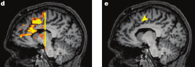
Figure 1 reproduced from Sheth et al (2012). d) dACC activation in response to conflict. e) arrow pointing to lesion site

Furthermore, the pattern of RTs before surgery followed a typical response pattern replicated over several studies using this task: RTs were faster for trials immediately following trials of a similar type - such as congruent trials following congruent trials, or incongruent trials following incongruent trials - and RTs were slower for trials which immediately followed trials of a different type, a pattern known as the Gratton effect.

The authors found that global error rates and RTs were similar before and after the surgery, dovetailing with the results reported by Fellows & Farah (2005); however, the modulation of RT based on previous trial congruency or incongruency was abolished. These results suggest that the ACC functions as a continuous updating mechanism modulating responses based on the weighted past and on trial-by-trial cognitive demands, which fits into the framework posited by Dosenbach (2007, 2008) that outlines the ACC as part of a rapid-updating cingulo-opercular network necessary for quick and flexible changes in performance based on task demands and performance history.

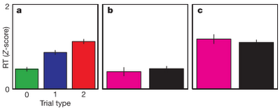
a) Pre-surgical RTs in response to trials of increasing conflict. b, c) Post-surgical RTs showing no difference between low-conflict trials preceded by either similar or different trial types (b), and no RT difference between high-conflict trials preceded by either similar or different trial types (c).

Above all, this experiment illustrates how lesion studies ought to be conducted. First, the authors identified a small population of subjects about to undergo a localized surgical procedure to lesion a specific area of the brain known to be involved in cognitive control; the same subjects were tested before the surgery using fMRI and during surgery using single-cell recordings; and interactions were tested which had been overlooked by previous lesion studies. It is an elegant and simple design; although I imagine that testing subjects while they had their skulls split open and electrodes jammed into their brains was disgusting. The things that these sickos will do for high-profile papers.

(This study may be profitably read in conjunction with a recent meta-analysis of lesion subjects (Gläscher et al, 2012; PNAS) dissociating cortical structures involved in cognitive control as opposed to decision-making and evaluation tasks. I recommend giving both of these studies a read.)